February 4, 2024 — Support my next blog post, buy me a coffee ☕.
In this post, I talk about an extension of the linear sampling method (LSM) for solving the sound-soft inverse acoustic scattering problem with data generated by randomly distributed small scatterers. For details, check out my paper with Houssem Haddar and Josselin Garnier!
Introduction
Inverse scattering problems arise across a multitude of fields, ranging from medical imaging and non-destructive testing to radar technology and seismology. At their core, these problems involve the task of deducing the characteristics of an object or medium from the scattered signals it generates. These problems involve several challenges, including nonlinearity, which is particularly pronounced near resonance, making linearization inapplicable; these are also severely ill-posed, raising questions about uniqueness and stability, and necessitating the inclusion of regularization. Additionally, for iterative procedures, reconstruction time can be lengthy and prior knowledge is required for initiation. In this context, fast, data-driven algorithms, such as the LSM, can be useful in reducing computational costs, and initializing more sophisticated algorithms.
Two acquisition configurations are commonly used in inverse scattering problems—active and passive. Active imaging involves sending waves through controlled sources and recording the medium's response through controlled sensors. Passive imaging, on the other hand, employs controlled sensors but relies on random, uncontrolled sources (such as microseisms and ocean swells in seismology). In this setup, it is the cross-correlations between the recorded signals that convey information about the medium. Passive imaging is a rapidly growing research topic because it enables the imaging of areas where the use of active sources is not possible due to, e.g., safety or environmental reasons. Additionally, even in scenarios where active sources could be employed, utilizing passive sources helps reduce operational costs and enhances stealth in defense applications.
In a previous paper, we introduced an extension of the LSM to address the sound-soft inverse scattering problem involving random sources. This current study builds upon that foundation, focusing on a scenario where a single controlled source, operating at a specified wavelength \(\lambda\), illuminates a small random scatterer and an object of comparable size to \(\lambda\)—the goal is to reconstruct the shape of the latter. The reflection of the wave field transmitted by the point source on the small scatterer serves as a random source, aligning with the context explored in our earlier work.
The motivation for this research stems from the necessity, when imaging an unknown obstacle \(D\), to illuminate it with a diverse set of incoming waves. For deterministic, controlled point sources, one considers a family of sources located at points \(\boldsymbol{z}_m\) generating the incident fields $$ \begin{align} \phi(\boldsymbol{x},\boldsymbol{z}_m) = \frac{i}{4}H_0^{(1)}(k\vert\boldsymbol{x}-\boldsymbol{z}_m\vert), \end{align} $$ and measures the resulting scattered fields \(u^s(\boldsymbol{x}_j,\boldsymbol{z}_m)\) at points \(\boldsymbol{x}_j\) to populate the near-field matrix \(N\) with entries \(N_{jm} = u^s(\boldsymbol{x}_j,\boldsymbol{z}_m)\). In the case of random, uncontrolled sources at positions \(\boldsymbol{z}_\ell\), as demonstrated in our prior work, the relevant matrix is the cross-correlation matrix \(C\). Its entries are given by: $$ \begin{align} C_{jm} = \frac{2ik\vert\Sigma\vert}{L}\sum_{\ell=1}^L\overline{u(\boldsymbol{x}_j,\boldsymbol{z}_\ell)}u(\boldsymbol{x}_m,\boldsymbol{z}_\ell) - \left[\phi(\boldsymbol{x}_j,\boldsymbol{x}_m) - \overline{\phi(\boldsymbol{x}_j,\boldsymbol{x}_m)}\right], \end{align} $$ where \(u(\boldsymbol{x},\boldsymbol{z})=\phi(\boldsymbol{x},\boldsymbol{z})+u^s(\boldsymbol{x},\boldsymbol{z})\) is the total field for the incident wave \(\phi(\boldsymbol{x},\boldsymbol{z})\), and \(\vert\Sigma\vert\) is the area of the surface \(\Sigma\) on which the random sources are distributed.
Suppose now that we only have a single controlled source located at some given point \(\boldsymbol{z}\), as opposed to several positions \(\boldsymbol{z}_m\). This is insufficient for reconstructing the obstacle's shape with the LSM (the near-field matrix \(N\) would have rank one). To address this limitation, we propose introducing a random medium between the source and the obstacle. We illustrate this concept, in acoustic scattering, by considering a single small random scatterer between the source and the obstacle—a seemingly simple yet powerful model of a random medium that allows us to apply the LSM in a novel manner, with a modified version of \(C\).
Modified Helmholtz–Kirchoff identity
Consider the incident field \(\phi(\boldsymbol{x},\boldsymbol{z}_\epsilon)\) generated by a point source located at \(\boldsymbol{z}_\epsilon=\lambda\epsilon^{-q}e^{i\theta_z}\) for some scalars \(\epsilon>0\), \(q>0\), and \(\theta_z\in[0,2\pi]\). Here, \(k>0\) is the wavenumber and \(\lambda=2\pi/k\) is the wavelength. Let \(D\) be an obstacle of size proportional to \(\lambda\) and independent on \(\epsilon\). Without loss of generality, we assume that \(D\) is centered at the origin. We also consider a small disk \(D_\epsilon=D_\epsilon(\boldsymbol{y}_\epsilon)\) of radius \(\rho(D_\epsilon)=\lambda\epsilon\) centered at \(\boldsymbol{y}_\epsilon = \lambda\epsilon^{-p}e^{i\theta_y}\) for some scalars \(0 < p < q\) and \(\theta_y\in[0,2\pi]\). Finally, let \(B\subset\mathbb{R}^2\setminus\overline{D\cup D_\epsilon}\) be a compact set whose size and distance to \(D\) are proportional to \(\lambda\) and independent on \(\epsilon\). Measurements will be taken inside the volume \(B\), which is consistent with our previous work.
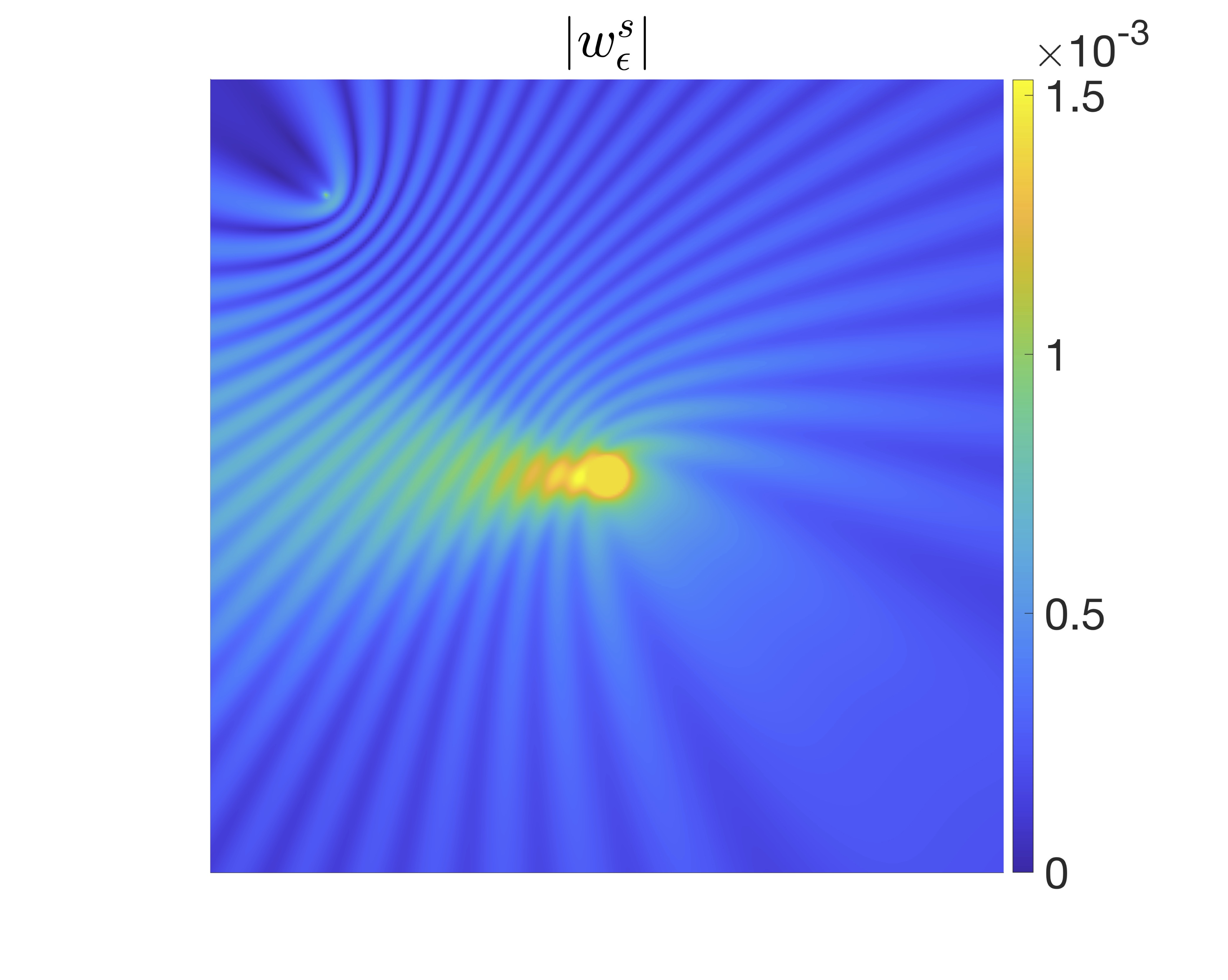
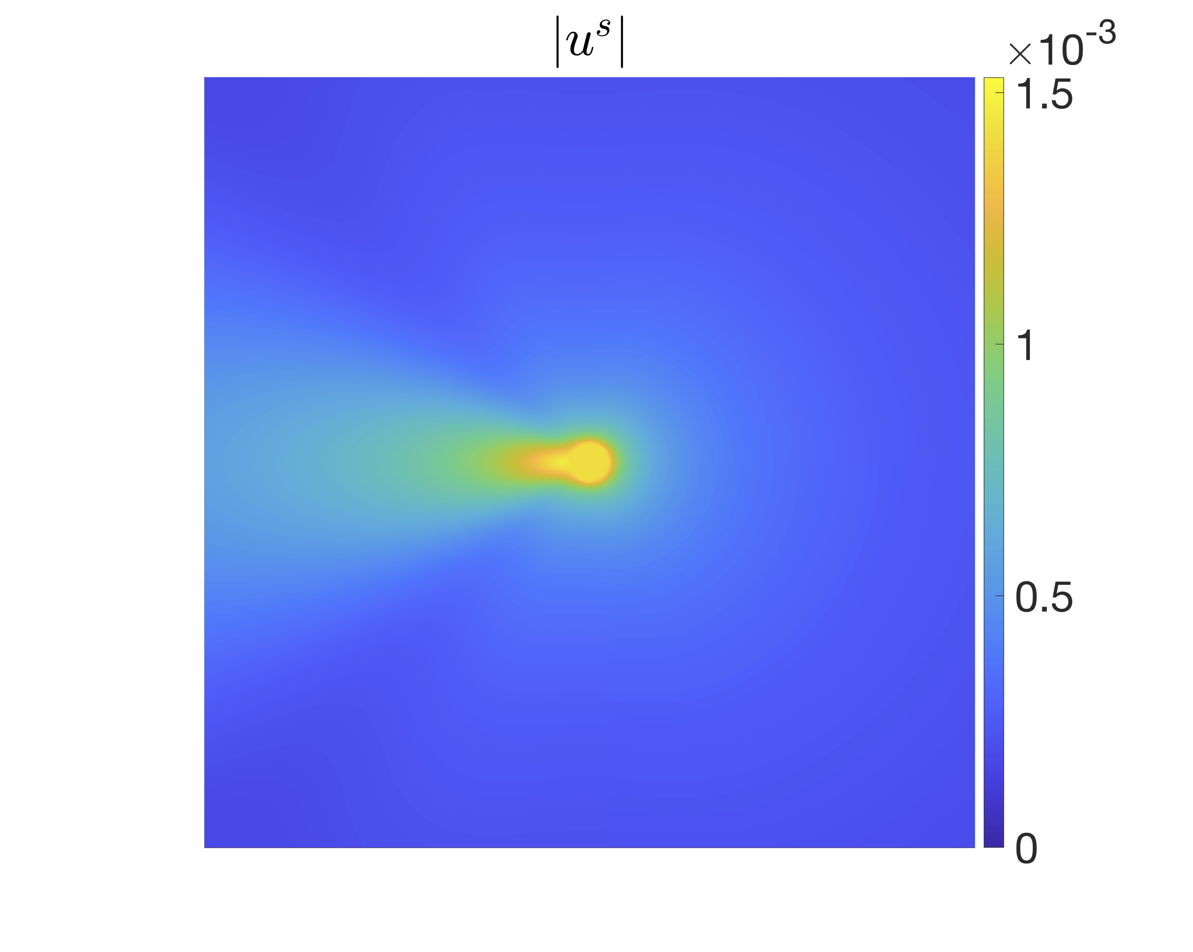
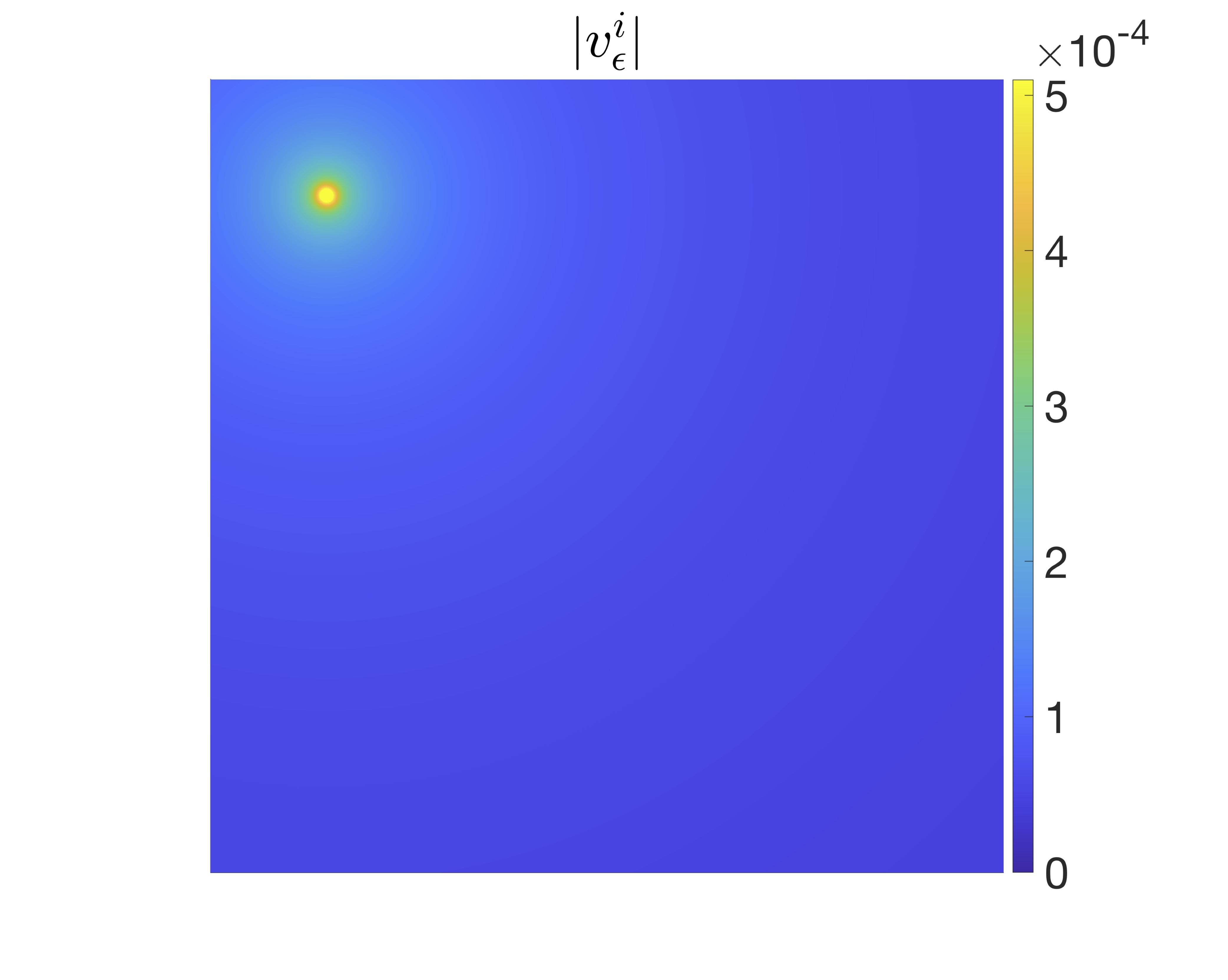
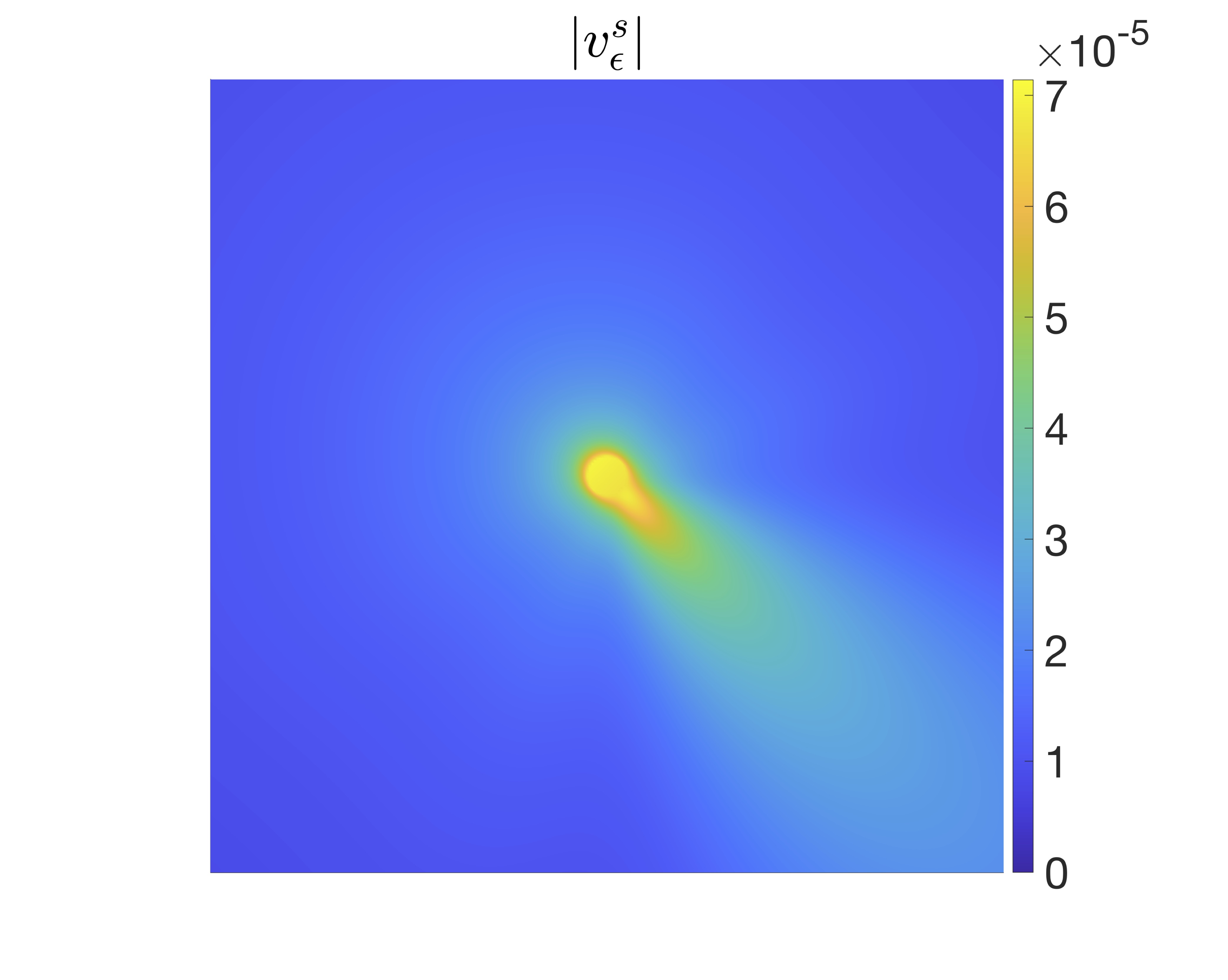
We examine the scattering of the incident field \(\phi(\cdot,\boldsymbol{z}_\epsilon)\) by \(D\) and \(D_\epsilon\), which generates the scattered field \(w^s_\epsilon\). More precisely, let \(w^s_\epsilon(\cdot,\boldsymbol{y}_\epsilon,\boldsymbol{z}_\epsilon)\) be the solution to the sound-soft scattering problem $$ \begin{align}\label{eq:w^s} \left\{ \begin{array}{ll} \Delta w^s_\epsilon(\cdot,\boldsymbol{y}_\epsilon,\boldsymbol{z}_\epsilon) + k^2 w^s_\epsilon(\cdot,\boldsymbol{y}_\epsilon,\boldsymbol{z}_\epsilon) = 0 \quad \text{in $\mathbb{R}^2\setminus\{\overline{D\cup D_\epsilon}\}$}, \\[0.4em] w^s_\epsilon(\cdot,\boldsymbol{y}_\epsilon,\boldsymbol{z}_\epsilon) = -\phi(\cdot,\boldsymbol{z}_\epsilon) \quad \text{on $\partial D\cup\partial D_\epsilon$}, \\[0.4em] \text{$w^s_\epsilon(\cdot,\boldsymbol{y}_\epsilon,\boldsymbol{z}_\epsilon)$ is radiating}. \end{array} \right. \end{align} $$ We showed that \(w^s_\epsilon(\cdot,\boldsymbol{y}_\epsilon,\boldsymbol{z}_\epsilon)\) may be approximated as the sum of three terms, $$ \begin{align} w_\epsilon^s(\cdot,\boldsymbol{y}_\epsilon,\boldsymbol{z}_\epsilon) \approx u^s(\cdot,\boldsymbol{z}_\epsilon) + v_\epsilon^i(\cdot,\boldsymbol{y}_\epsilon,\boldsymbol{z}_\epsilon) + v_\epsilon^s(\cdot,\boldsymbol{y}_\epsilon,\boldsymbol{z}_\epsilon) \end{align} $$ with an error \(\mathcal{O}(\vert\log\epsilon\vert^{-1}\epsilon^p\epsilon^{q/2})\) in the \(H^1(B)\)-norm; the scattered fields in the expansion above are the solutions to the sound-soft scattering problems $$ \begin{align}\label{eq:u^s} \left\{ \begin{array}{ll} \Delta u^s(\cdot,\boldsymbol{z}_\epsilon) + k^2 u^s(\cdot,\boldsymbol{z}_\epsilon) = 0 \quad \text{in $\mathbb{R}^2\setminus\overline{D}$}, \\[0.4em] u^s(\cdot,\boldsymbol{z}_\epsilon) = -\phi(\cdot,\boldsymbol{z}_\epsilon) \quad \text{on $\partial D$}, \\[0.4em] \text{$u^s(\cdot,\boldsymbol{z}_\epsilon)$ is radiating}, \end{array} \right. \end{align} $$ $$ \begin{align}\label{eq:v^i} \left\{ \begin{array}{ll} \Delta v_\epsilon^i(\cdot,\boldsymbol{y}_\epsilon,\boldsymbol{z}_\epsilon) + k^2 v_\epsilon^i(\cdot,\boldsymbol{y}_\epsilon,\boldsymbol{z}_\epsilon) = 0 \quad \text{in $\mathbb{R}^2\setminus\overline{D_\epsilon}$}, \\[0.4em] v_\epsilon^i(\cdot,\boldsymbol{y}_\epsilon,\boldsymbol{z}_\epsilon) = -\phi(\cdot,\boldsymbol{z}_\epsilon) \quad \text{on $\partial D_\epsilon$}, \\[0.4em] \text{$v_\epsilon^i(\cdot,\boldsymbol{y}_\epsilon,\boldsymbol{z}_\epsilon)$ is radiating}, \end{array} \right. \end{align} $$ and $$ \begin{align}\label{eq:v^s} \left\{ \begin{array}{ll} \Delta v_\epsilon^s(\cdot,\boldsymbol{y}_\epsilon,\boldsymbol{z}_\epsilon) + k^2 v_\epsilon^s(\cdot,\boldsymbol{y}_\epsilon,\boldsymbol{z}_\epsilon) = 0 \quad \text{in $\mathbb{R}^2\setminus\overline{D}$}, \\[0.4em] v_\epsilon^s(\cdot,\boldsymbol{y}_\epsilon,\boldsymbol{z}_\epsilon) = -v^i_\epsilon(\cdot,\boldsymbol{y}_\epsilon,\boldsymbol{z}_\epsilon) \quad \text{on $\partial D$}, \\[0.4em] \text{$v_\epsilon^s(\cdot,\boldsymbol{y}_\epsilon,\boldsymbol{z}_\epsilon)$ is radiating}. \end{array} \right. \end{align} $$
This is how the scattered fields look like.
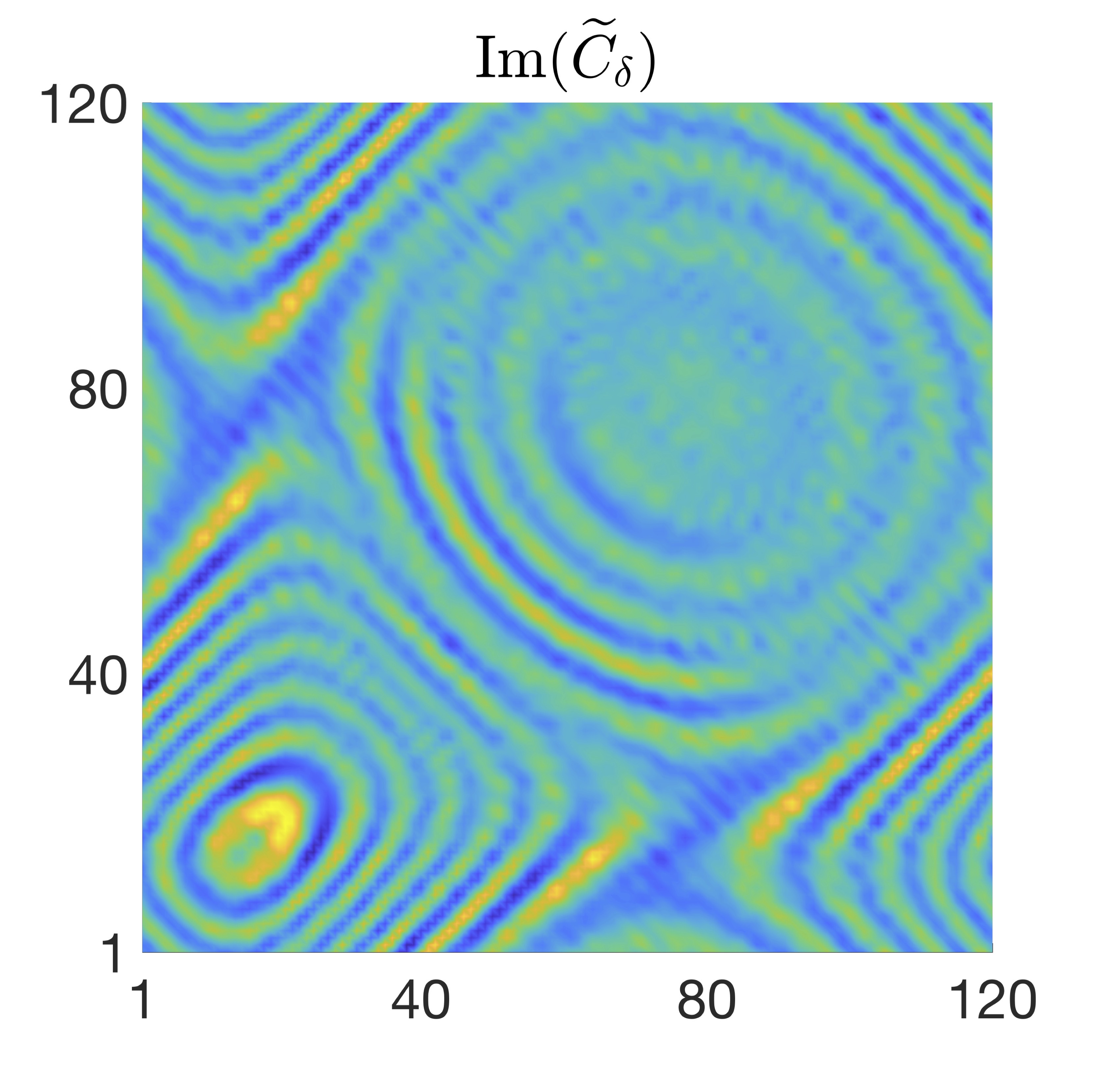
We proved that the scattered fields verify the following modified Helmholtz–Kirchhoff identity, $$ \begin{align} u^s(\boldsymbol{x},\boldsymbol{x}') - \overline{u^s(\boldsymbol{x},\boldsymbol{x}')} \approx 2ik\sigma_\epsilon\int_{\Sigma_\epsilon}\overline{v_\epsilon(\boldsymbol{x},\boldsymbol{y}_\epsilon,\boldsymbol{z}_\epsilon)} v_\epsilon(\boldsymbol{x}',\boldsymbol{y}_\epsilon,\boldsymbol{z}_\epsilon)dS(\boldsymbol{y}_\epsilon) - [\phi(\boldsymbol{x},\boldsymbol{x}') - \overline{\phi(\boldsymbol{x},\boldsymbol{x}')}], \end{align} $$ with scaling factor \(\sigma_\epsilon = \pi^2\vert H_0^{(1)}(2\pi\epsilon)\vert^2\epsilon^{-q}\). This motivates the introduction of the following modified cross-correlation matrix: $$ \begin{align} \widetilde{C}_{jm} = \frac{2ik\vert\Sigma_\epsilon\vert\sigma_\epsilon}{L}\sum_{\ell=1}^L\overline{v_\epsilon(\boldsymbol{x}_j,\boldsymbol{y}_\epsilon^\ell,\boldsymbol{z}_\epsilon)} v_\epsilon(\boldsymbol{x}_m,\boldsymbol{y}_\epsilon^\ell,\boldsymbol{z}_\epsilon) - \left[\phi(\boldsymbol{x}_j,\boldsymbol{x}_m) - \overline{\phi(\boldsymbol{x}_j,\boldsymbol{x}_m)}\right]. \end{align} $$
Numerical experiments
We consider a kite of size \(\lambda/2\) centered at \(2\lambda + 2\lambda i\) for the wavenumber \(k=2\pi\) (wavelength \(\lambda =1\)). We take \(\epsilon=10^{-2}\), \(p=1\), \(q=2\), and \(\theta_z=\pi\) for the asymptotic model, which yields \(\boldsymbol{z}_\epsilon=-10000\). For the LSM, we take \(J=120\) equispaced sensors on the circle of radius \(5\lambda=5\), $$ \begin{align} \boldsymbol{x}_j = 5e^{i\theta_j}, \quad \theta_j = \frac{2\pi}{J}(j - 1), \quad 1\leq j\leq J, \end{align} $$ and \(L=120\) different positions of a single small scatterer on the circle of radius \(\lambda\epsilon^{-p}=100\), \begin{align}\label{eq:scatterer-beta} \boldsymbol{y}_\epsilon^\ell = 100e^{i\theta_y^\ell}, \quad \theta_y^\ell = 2\pi\beta_\ell, \quad 1\leq \ell\leq L, \end{align} where \(\beta_\ell\sim U(0,1)\) is drawn from the uniform distribution on \([0,1]\). Finally, we add some multiplicative white noise with amplitude \(\delta=5\times 10^{-3}\) to the the near-field measurements (generating a matrix \(\widetilde{C}_\delta\)), and probe the medium on a \(100\times100\) uniform grid on \([-6\lambda,6\lambda]\times[-6\lambda,6\lambda]\).
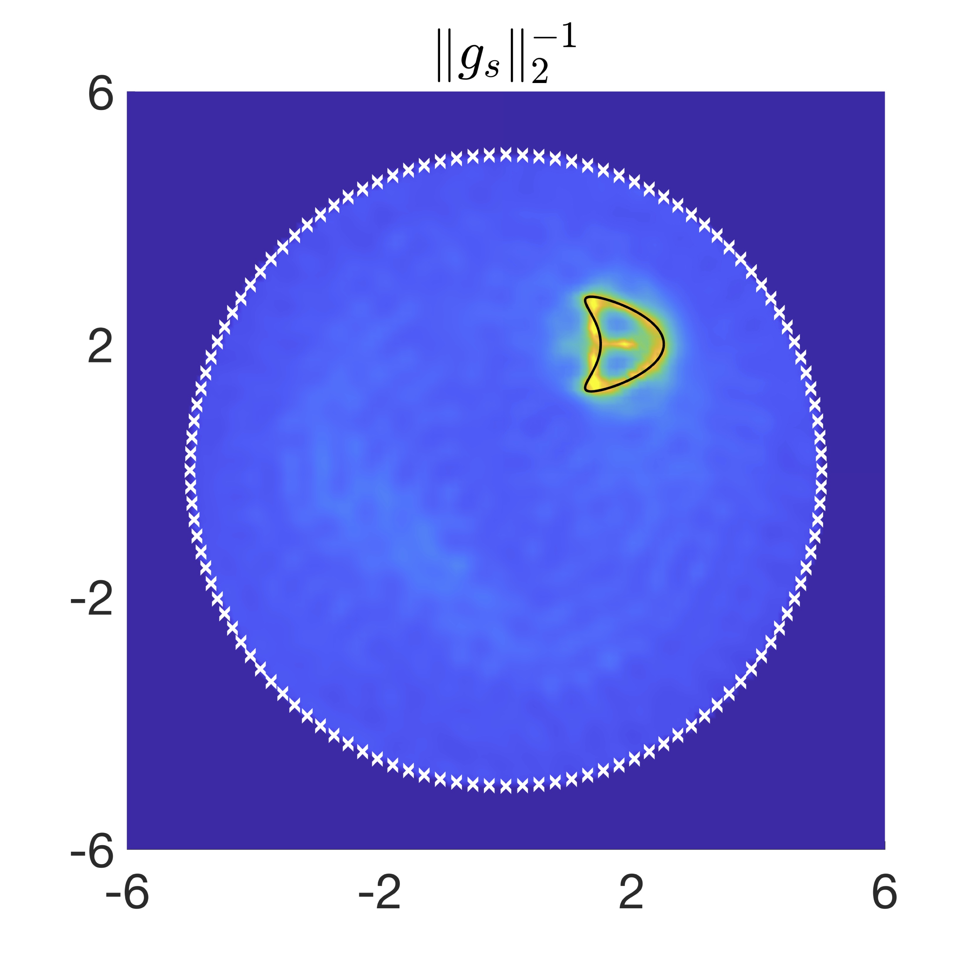
The defect is well identified by our novel sampling method, based on cross-correlations and a small random scatterer. This illustrates that the LSM can be utilized in this novel passive-imaging setup.