November 4, 2022
In this post, I talk about an extension of the linear sampling method (LSM) for solving the sound-soft inverse acoustic scattering problem with randomly distributed point sources. For details, check out my paper with Houssem Haddar and Josselin Garnier!
Introduction
A typical inverse scattering problem is the identification of the shape of a defect inside a medium by sending waves that propagate within. In the data acquisition step, several receivers record the medium's response that forms the data of the inverse problem; in the data processing step, numerical algorithms are used to recover an approximation of the shape from the measurements. What we have just described is an example of active imaging, where both the sources and the receivers are controlled. In passive imaging, only receivers are employed and the illumination comes from uncontrolled, random sources. In this setup, it is the cross-correlations between the recorded signals that convey information about the medium through which the waves propagate.
The Helmholtz–Kirchoff identity
Acoustic scattering is governed by the Helmholtz equation \(\Delta u+k^2u=0\), whose Green's function is $$ \phi(\boldsymbol{x},\boldsymbol{y}) = \frac{i}{4}H_0^{(1)}(k\vert\boldsymbol{x}-\boldsymbol{y}\vert) $$ in dimension two and $$ \quad \phi(\boldsymbol{x},\boldsymbol{y}) = \frac{e^{ik\vert\boldsymbol{x}-\boldsymbol{y}\vert}}{4\pi \vert\boldsymbol{x}-\boldsymbol{y}\vert} $$ in dimension three. The number \(k>0\) is the wavenumber (the wavelength is \(\lambda=2\pi/k\)), and \(i\) denotes the imaginary unit. The Helmholtz–Kirchhoff identity for the Green's function reads $$ \phi(\boldsymbol{x},\boldsymbol{y}) - \overline{\phi(\boldsymbol{x},\boldsymbol{y})} = 2ik\int_{\Sigma}\overline{\phi(\boldsymbol{x},\boldsymbol{z})}\phi(\boldsymbol{y},\boldsymbol{z})dS(\boldsymbol{z}), $$ where the surface \(\Sigma\) encloses \(\boldsymbol{x}\) and \(\boldsymbol{y}\). The identity above connects the imaginary part of the measurements at \(\boldsymbol{x}\) of point sources located at \(\boldsymbol{y}\) (left) to the cross-correlation between the measurements at \(\boldsymbol{x}\) and \(\boldsymbol{y}\) of point sources on \(\Sigma\) (right).
The Helmholtz–Kirchhoff identity applies to total fields, too. Let \(D\subset\mathbb{R}^d\) (for \(d=2\) or 3) be a bounded domain whose complement is connected and \(\boldsymbol{y}\in\mathbb{R}^d\). A point source located at \(\boldsymbol{y}\in\mathbb{R}^d\setminus\overline{D}\) transmits a time-harmonic signal that generates the incident field \(\phi(\cdot,\boldsymbol{y})\). The scattered field \(u^s(\cdot,\boldsymbol{y})\) for a sound-soft defect \(D\) is the solution to $$ \left\{ \begin{array}{ll} \Delta u^s(\cdot,\boldsymbol{y}) + k^2 u^s(\cdot,\boldsymbol{y}) = 0 \quad \text{in $\mathbb{R}^d\setminus\overline{D}$}, \\[0.4em] \phi(\cdot,\boldsymbol{y}) + u^s(\cdot,\boldsymbol{y}) = 0 \quad \text{on $\partial D$}, \\[0.4em] \text{$u^s(\cdot,\boldsymbol{y})$ is radiating}. \end{array} \right. $$ The total field is then defined as \(u(\boldsymbol{x},\boldsymbol{y})=\phi(\boldsymbol{x},\boldsymbol{y})+u^s(\boldsymbol{x},\boldsymbol{y})\). The Helmholtz–Kirchhoff identity for total fields is: $$ u(\boldsymbol{x},\boldsymbol{y}) - \overline{u(\boldsymbol{x},\boldsymbol{y})} = 2ik\int_{\Sigma}\overline{u(\boldsymbol{x},\boldsymbol{z})}u(\boldsymbol{y},\boldsymbol{z})dS(\boldsymbol{z}). $$ This immediately implies the following relationship for the scattered fields, $$ \begin{align} u^s(\boldsymbol{x},\boldsymbol{y}) - \overline{u^s(\boldsymbol{x},\boldsymbol{y})} = 2ik\int_{\Sigma}\overline{u(\boldsymbol{x},\boldsymbol{z})}u(\boldsymbol{y},\boldsymbol{z})dS(\boldsymbol{z}) - \left[\phi(\boldsymbol{x},\boldsymbol{y}) - \overline{\phi(\boldsymbol{x},\boldsymbol{y})}\right]. \end{align} $$
The standard LSM in active imaging
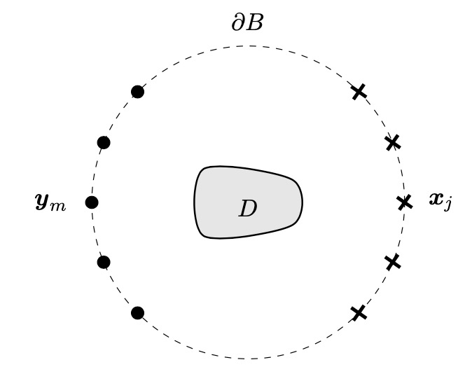
Let \(\boldsymbol{x}_j\), \(1\leq j\leq J\), and \(\boldsymbol{y}_m\), \(1\leq m\leq M\), be measurement points and point sources located on a surface \(\partial B\) that encloses \(D\). The standard LSM for near-field measurements, in active imaging, relies on the construction of the near-field matrix \(N^\mathrm{ac}\) with entries $$ N^\mathrm{ac}_{jm} = u^s(\boldsymbol{x}_j,\boldsymbol{y}_m). $$ The matrix \(N^\mathrm{ac}\) corresponds to the medium's response, measured at \(\boldsymbol{x}_j\), to the illumination by point sources located at \(\boldsymbol{y}_m\). Here, the positions of both measurement points and point sources are known and controlled. This matrix is filled out in the data acquisition step, which entails the solution of the PDE for each \(\boldsymbol{y}_m\). In the processing step, we numerically probe the medium by solving the linear system \(N^\mathrm{ac}g_{\boldsymbol{z}}=\phi_{\boldsymbol{z}}\) for various \(\boldsymbol{z}\in\mathbb{R}^d\). (The right-hand side is defined by \((\phi_{\boldsymbol{z}})_j = \phi(\boldsymbol{x}_j, \boldsymbol{z})\), \(1\leq j\leq J\).) The boundary \(\partial D\) of the defect \(D\) coincides with those points \(\boldsymbol{z}\) for which the value of \(\Vert g_{\boldsymbol{z}}\Vert_2\) is large. The setup we have described is shown below.
The new LSM for passive imaging
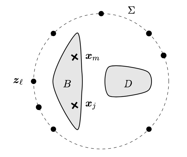
In passive imaging, we assume that the measurement points \(\boldsymbol{x}_j\) are located in some bounded volume \(B\subset\mathbb{R}^d\setminus\overline{D}\). Let \(\Sigma\) be a surface that encloses \(B\) and \(D\), and let us assume that there are \(L>0\) point sources \(\boldsymbol{z}_\ell\) randomly distributed on \(\Sigma\). These sources can transmit a unit-amplitude time-harmonic signal, one by one, so that it is possible to measure the total fields \(u(\boldsymbol{x}_j,\boldsymbol{z}_\ell)\). Moreover, it is possible to compute \(\phi(\boldsymbol{x}_j,\boldsymbol{x}_m)\), so we can evaluate the cross-correlation matrix \(C\) with entries $$ \begin{align} C_{jm} = \frac{2ik\vert\Sigma\vert}{L}\sum_{\ell=1}^L\overline{u(\boldsymbol{x}_j,\boldsymbol{z}_\ell)}u(\boldsymbol{x}_m,\boldsymbol{z}_\ell) - \left[\phi(\boldsymbol{x}_j,\boldsymbol{x}_m) - \overline{\phi(\boldsymbol{x}_j,\boldsymbol{x}_m)}\right], \end{align} $$ where \(\vert\Sigma\vert\) is the area of \(\Sigma\). The matrix \(C\) corresponds to the discretization of the right-hand side of the Helmholtz–Kirchhoff identity (for scattered fields) at points \(\boldsymbol{z}_\ell\) with uniform weights and evaluted at \(\boldsymbol{x}_j\) and \(\boldsymbol{x}_m\), i.e., $$ \begin{align} C_{jm} \approx 2ik\int_{\Sigma}\overline{u(\boldsymbol{x}_j,\boldsymbol{z})}u(\boldsymbol{x}_m,\boldsymbol{z})dS(\boldsymbol{z}) - \left[\phi(\boldsymbol{x}_j,\boldsymbol{x}_m) - \overline{\phi(\boldsymbol{x}_j,\boldsymbol{x}_m)}\right]. \end{align} $$ Therefore, it satisfies $$ C_{jm} \approx N_{jm} - \overline{N_{jm}}, $$ where the matrix \(N\) is the standard near-field matrix for co-located receivers and sources: $$ N_{jm} = u^s(\boldsymbol{x}_j,\boldsymbol{x}_m). $$ This motivates the introduction of the imaginary near-field matrix \(I\), $$ I_{jm} = N_{jm} - \overline{N_{jm}} = u^s(\boldsymbol{x}_j,\boldsymbol{x}_m) - \overline{u^s(\boldsymbol{x}_j,\boldsymbol{x}_m)}. $$ In our paper, we justified the utilization of the matrix \(I\) for the LSM in active imaging. If the LSM works for \(I\) in active imaging, then, via the Helmholtz–Kirchhoff identity \(C_{jm} \approx I_{jm}\), it works for \(C\) in passive imaging. The setup we have described is shown below.
Numerical experiments
We consider the scattering of points sources by a kite of size \(\lambda/2\) centered at \(2\lambda + 2\lambda i\) for \(k=2\pi\) (wavelength \(\lambda =1\)). We compare the results obtained for the near-field matrix \(N\), the imaginary near-field matrix \(I\), and the cross-correlation matrix \(C\). For \(N\) and \(I\), we take \(J=80\) equispaced co-located sources and receivers on the circle of radius \(5\lambda\), $$ \boldsymbol{x}_j = 5\lambda e^{i\theta_j}, \quad \theta_j = \frac{2\pi}{J}(j - 1). $$ For the matrix \(C\), the \(L=80\) random sources are located on the circle of radius \(50\lambda\), $$ \boldsymbol{z}_\ell = 50\lambda e^{i\theta_\ell}, \quad \theta_\ell = \frac{2\pi}{L}(\ell -1+ \beta_\ell), $$ where \(\beta_\ell\) is drawn from the uniform distribution on \([0,\beta]\) with \(\beta=0.1\), and we measure at the points \(\boldsymbol{x}_j\). To simulate noisy measurements, we add some white noise of amplitude \(5\times 10^{-2}\) to each matrix; we call the noisy matrices \(N_\delta\), \(I_\delta\), and \(C_\delta\). Finally, we probe the medium on a \(100\times100\) uniform grid on \([-6\lambda,6\lambda]\times[-6\lambda,6\lambda]\). Here are the results.
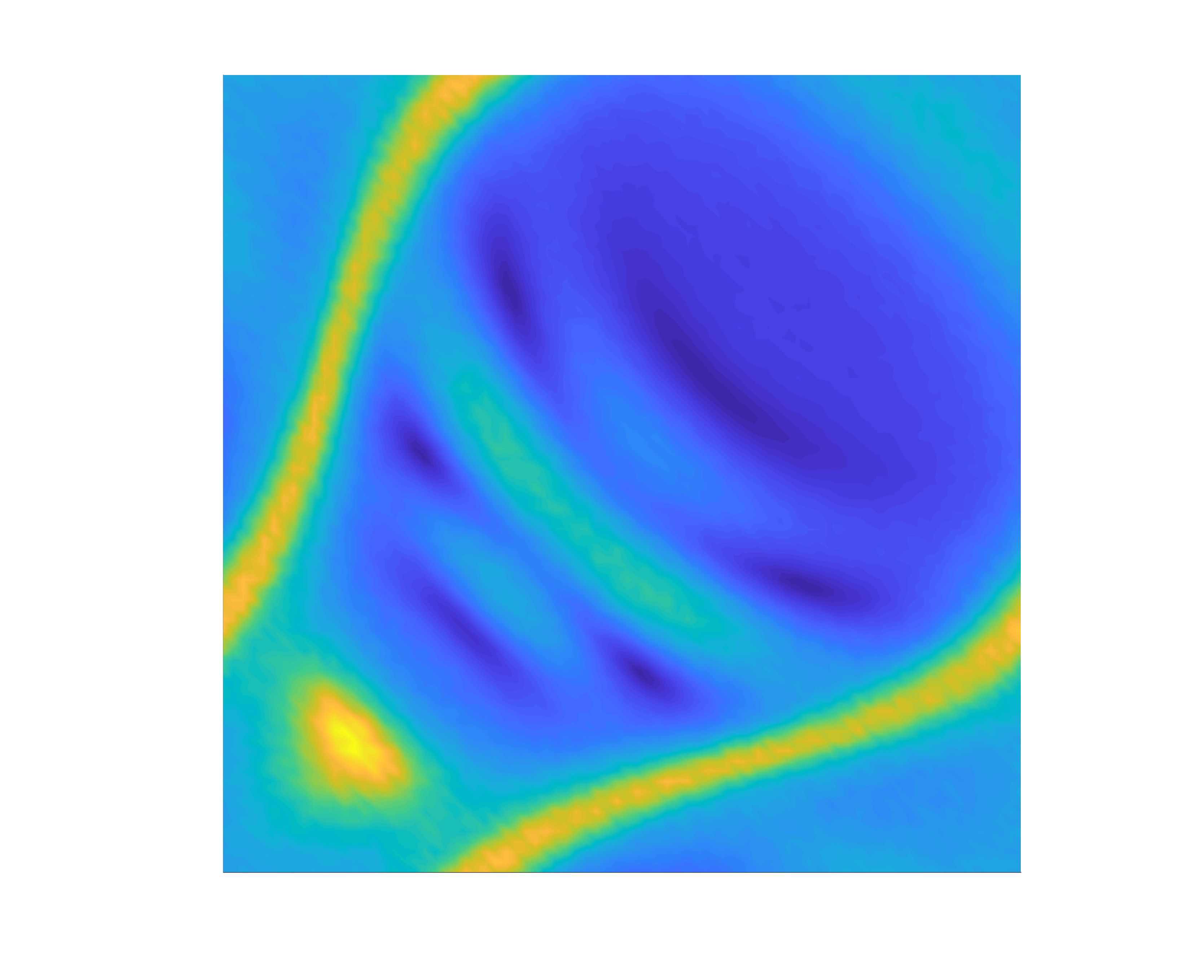
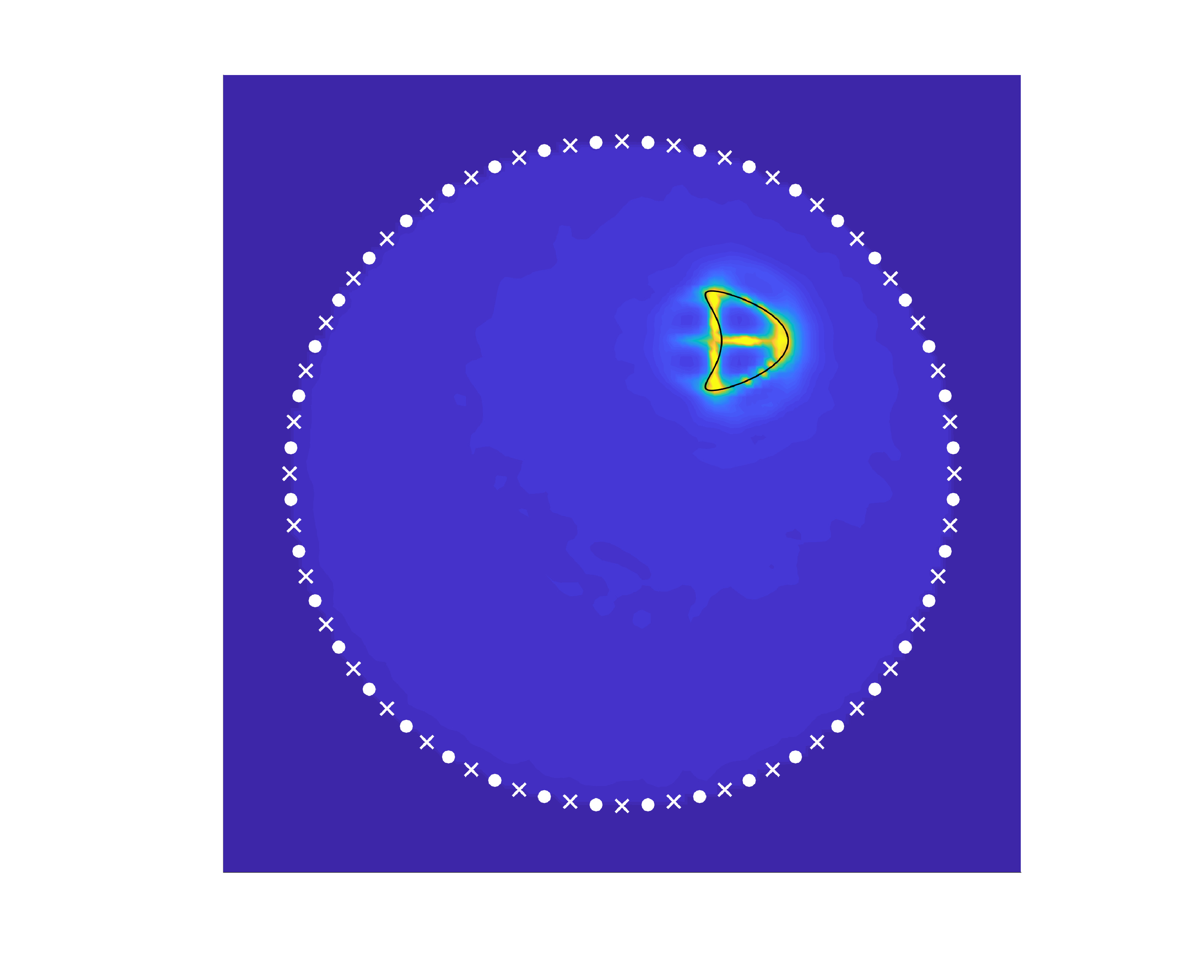
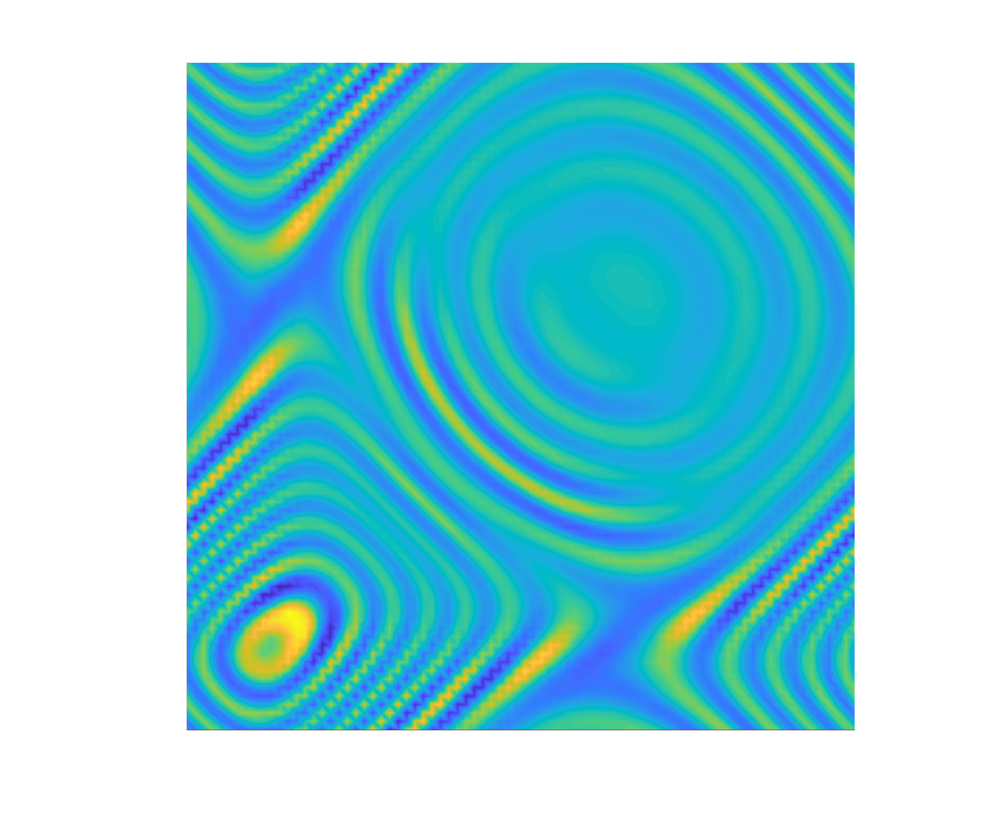
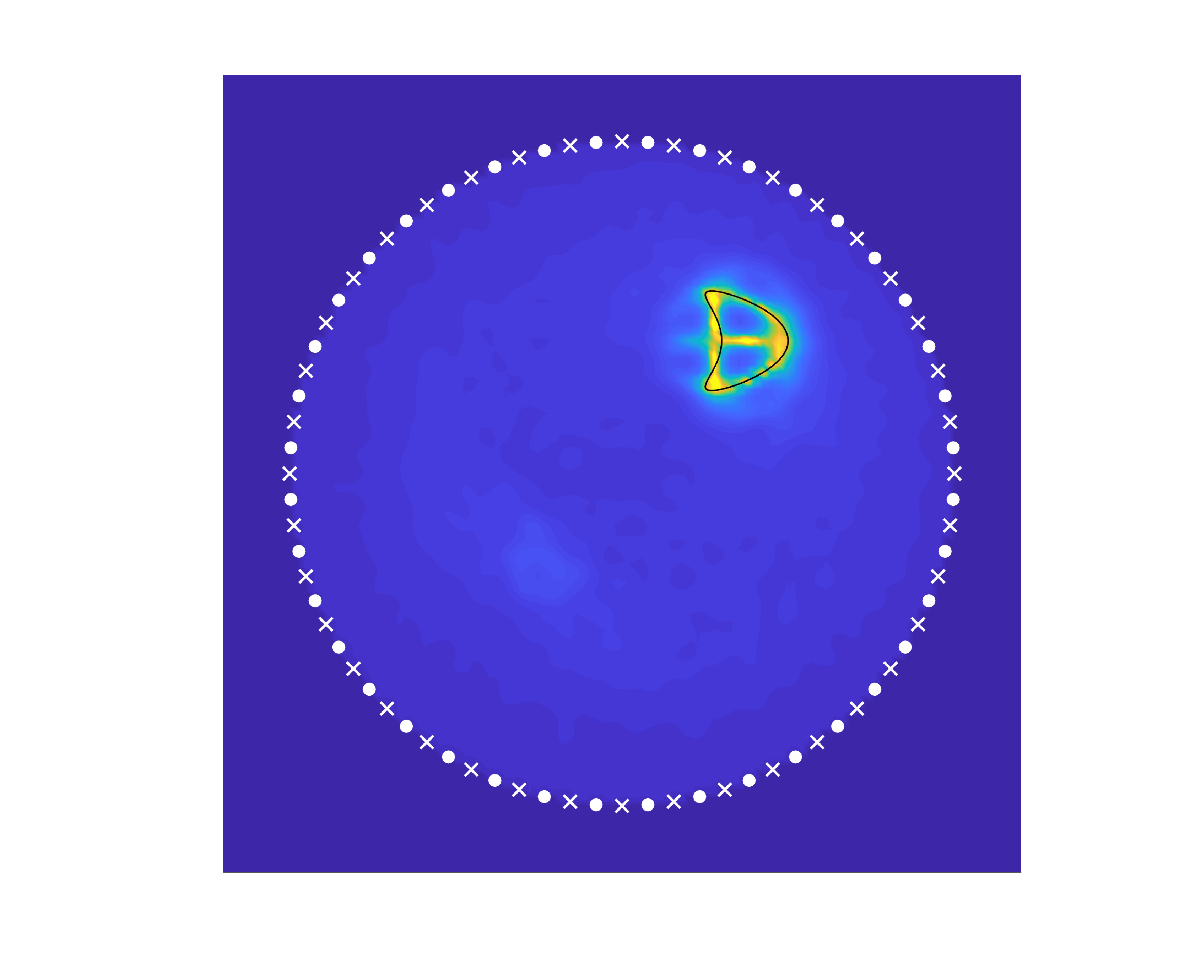
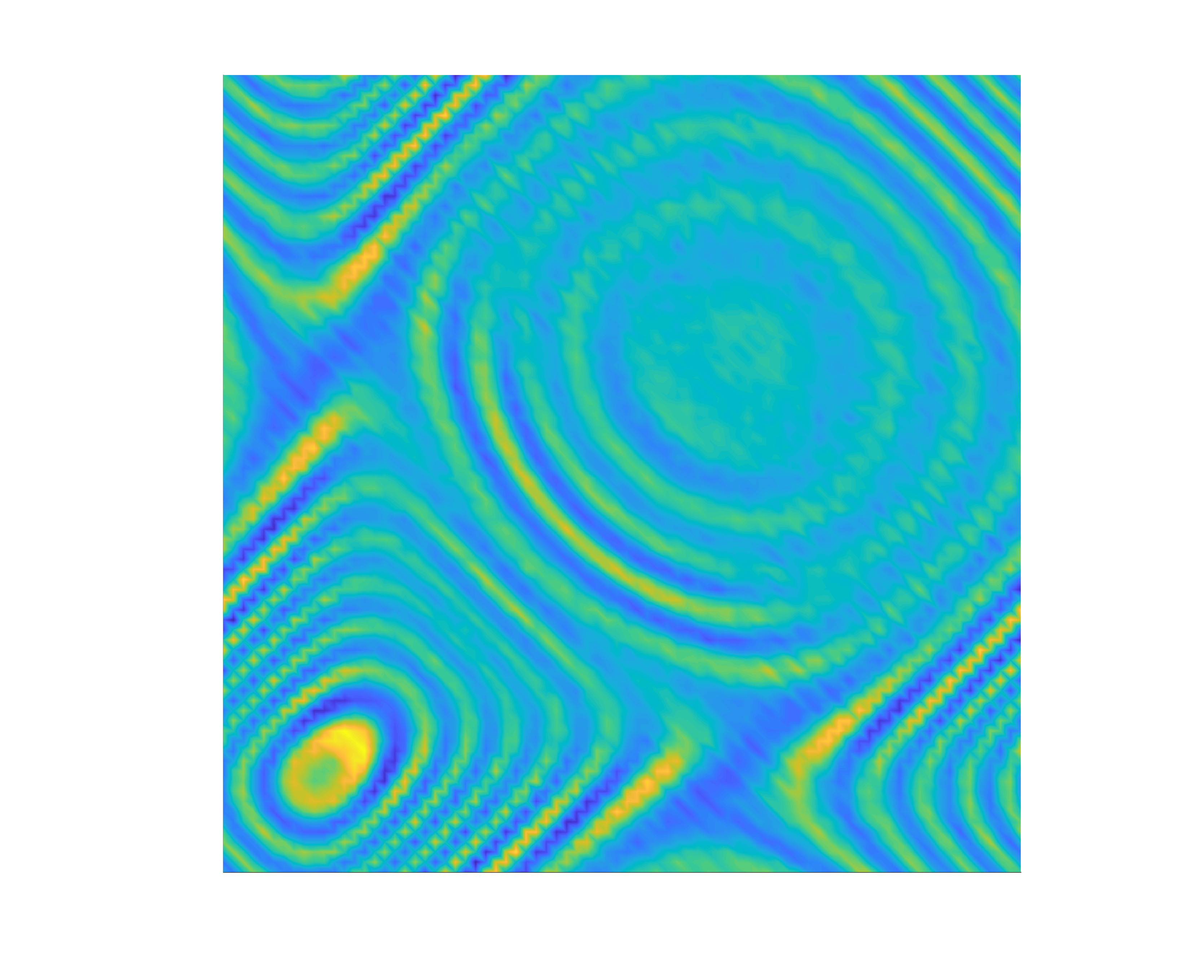
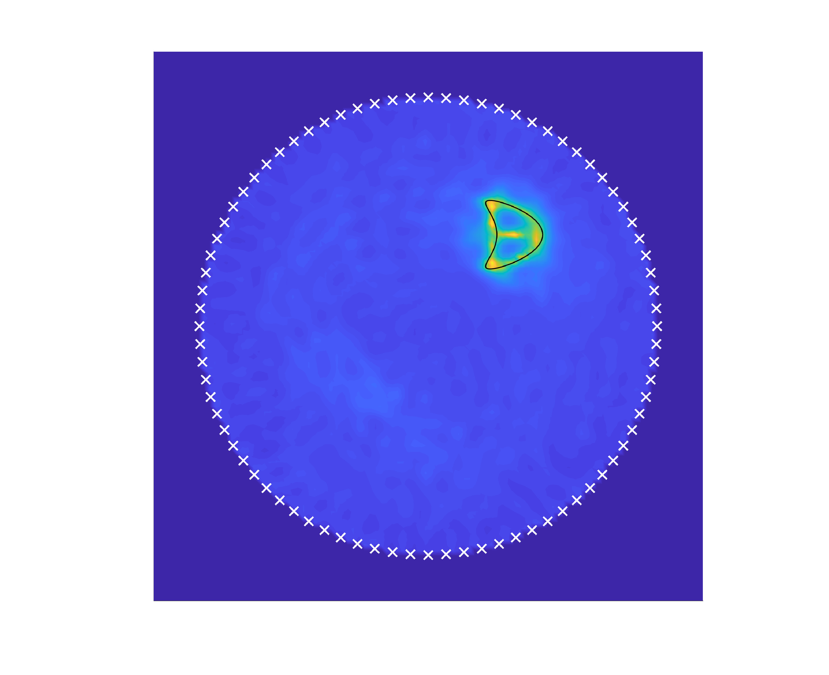
The first column displays the matrices and the second column the indicator function (values outside of the circle of radius \(5\lambda\) were zeroed out). The sources are represented by dots, and the measurement points by crosses. For \(N\) and \(I\), we plotted every other source/measurement point; for \(C\), the random sources are outside of the plot. Our novel LSM (third row), based on cross-correlations and random sources, shows similar results to the LSM with deterministic sources (first row). The LSM can be utilized in passive imaging!