December 30, 2022
In this post, I talk about image and video matting—the process of extracting specific objects from an image to place them in a scene of a movie or compose them onto another background.
Introduction
Formally, matting techniques take as input in image \(I\), which is assumed to be a convex combination of a foreground image \(F\) and a background image \(B\), $$ I = \alpha F + (1-\alpha)B, $$ where \(\alpha\) is the pixel's foreground opacity or matte. The above equation applies to each pixel of the image \(I\) and for each RGB component of this pixel. In other words, the above equation is an identity between vectors, which we can write as $$ \begin{bmatrix}\mathrm{R}_I\\\mathrm{G}_I\\\mathrm{B}_I\end{bmatrix} = \alpha\begin{bmatrix}\mathrm{R}_F\\\mathrm{G}_F\\\mathrm{B}_F\end{bmatrix} + (1-\alpha)\begin{bmatrix}\mathrm{R}_B\\\mathrm{G}_B\\\mathrm{B}_B\end{bmatrix} \quad\text{at each pixel}. $$ This is what we call the matting equation. Here, the input image \(I\) is given and the matte \(\alpha\) and the foreground and background images \(F\) and \(B\) are unknowns, that is, we have seven variables $$ (\mathrm{R}_F,\mathrm{G}_F,\mathrm{B}_F,\mathrm{R}_B,\mathrm{G}_B,\mathrm{B}_B,\alpha) $$ but only three equations—one per RGB component. (More precisely, if the image is \(N\times N\), we have \(7N^2\) variables and \(3N^2\) equations.) Mathematically, we say that this set of equations is underdetermined. There is no general and obvious way to solve it unless we make some simplifying assumptions or else are given some additional inputs.
Green screen matting
In green screen matting, also called chroma keying, we assume that the background image \(B\) is a given uniform green color \(\mathrm{G}_B\). In terms of RGB components, this means that $$ B = \begin{bmatrix}0\\\mathrm{G}_B\\0\end{bmatrix}. $$ In this case, the matting equation simplifies to $$ \begin{bmatrix}\mathrm{R}_I\\\mathrm{G}_I\\\mathrm{B}_I\end{bmatrix} = \alpha\begin{bmatrix}\mathrm{R}_F\\\mathrm{G}_F\\\mathrm{B}_F\end{bmatrix} + (1-\alpha)\begin{bmatrix}0\\\mathrm{G}_B\\0\end{bmatrix}. $$ We now have four variables \((\mathrm{R}_F,\mathrm{G}_F,\mathrm{B}_F,\alpha)\) and three equations—this is a much simpler problem. We can even obtain exact solutions in several specific cases.
Gray images
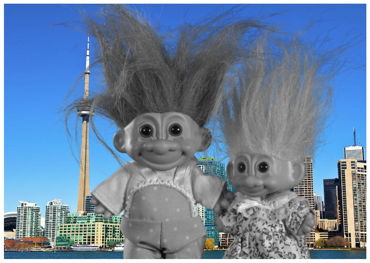
For gray foreground images \(F\), we may assume that $$ \mathrm{R}_F = \mathrm{G}_F = \mathrm{B}_F, $$ which leads to $$ \begin{bmatrix}\mathrm{R}_I\\\mathrm{G}_I\\\mathrm{B}_I\end{bmatrix} = \alpha\begin{bmatrix}\mathrm{R}_F\\\mathrm{R}_F\\\mathrm{R}_F\end{bmatrix} + (1-\alpha)\begin{bmatrix}0\\\mathrm{G}_B\\0\end{bmatrix}. $$ In this case, we only have two variables \((\mathrm{R}_F,\alpha)\). The three equations read $$ \left\{ \begin{array}{ll} \mathrm{R}_I = \alpha\mathrm{R}_F, \\ \mathrm{G}_I = \alpha\mathrm{R}_F + (1-\alpha)\mathrm{G}_B, \\ \mathrm{B}_I = \alpha\mathrm{R}_F. \end{array} \right. $$ The first and third equations yield $$ \alpha\mathrm{R}_F = \mathrm{R}_I = \mathrm{B}_I,$$ while the second equation gives \(\mathrm{G}_I = \mathrm{R}_I + (1-\alpha)\mathrm{G}_B\), that is, $$ \alpha = \frac{\mathrm{R}_I - (\mathrm{G}_I - \mathrm{G}_B)}{\mathrm{G}_B}. $$ To obtain a new image \(J\) with a different background \(K\), one can simply compute $$ J = \alpha F +(1-\alpha)K, $$ that is, $$ \begin{align} \begin{bmatrix}\mathrm{R}_J\\\mathrm{G}_J\\\mathrm{B}_J\end{bmatrix} = \alpha\begin{bmatrix}\mathrm{R}_F\\\mathrm{R}_F\\\mathrm{R}_F\end{bmatrix} + (1-\alpha)\begin{bmatrix}\mathrm{R}_K\\\mathrm{G}_K\\\mathrm{B}_K\end{bmatrix} = \begin{bmatrix}\mathrm{R}_I\\\mathrm{R}_I\\\mathrm{R}_I\end{bmatrix} +(1-\alpha)\begin{bmatrix}\mathrm{R}_K\\\mathrm{G}_K\\\mathrm{B}_K\end{bmatrix}. \end{align} $$
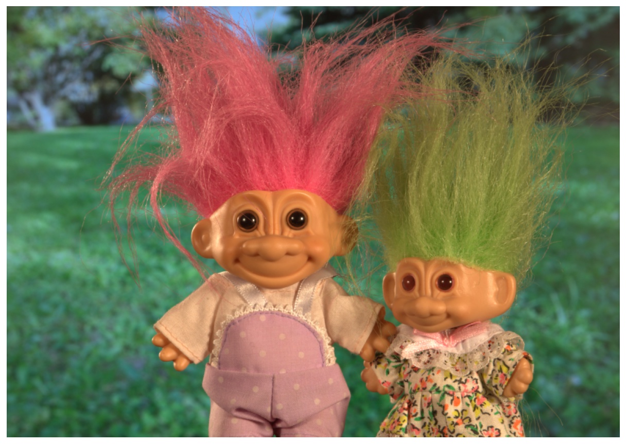
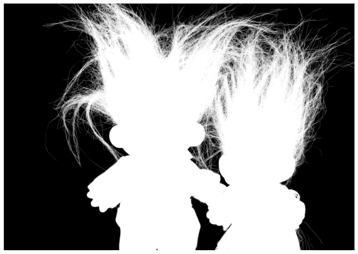
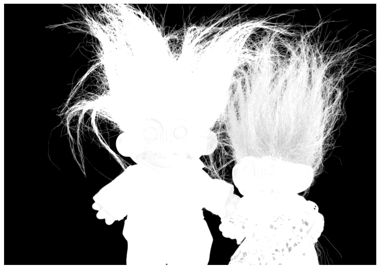
Let's look at an example. Consider the following image from the alpha matting evaluation website together with its "exact" matte:
import cv2
import matplotlib.pyplot as plt
import numpy as np

I = cv2.imread('GT04.png')                                         # load image I (BGR format)
I = cv2.cvtColor(I, cv2.COLOR_BGR2RGB)/255                         # convert to RGB and normalize
plt.imshow(I), plt.axis('off')                                     # plot I
plt.show();
alpha_ex = cv2.imread('GT04_alpha.png', cv2.IMREAD_GRAYSCALE)/255  # load exact alpha and normalize
plt.imshow(alpha_ex, cmap='gray'), plt.axis('off')                 # plot alpha
plt.show();
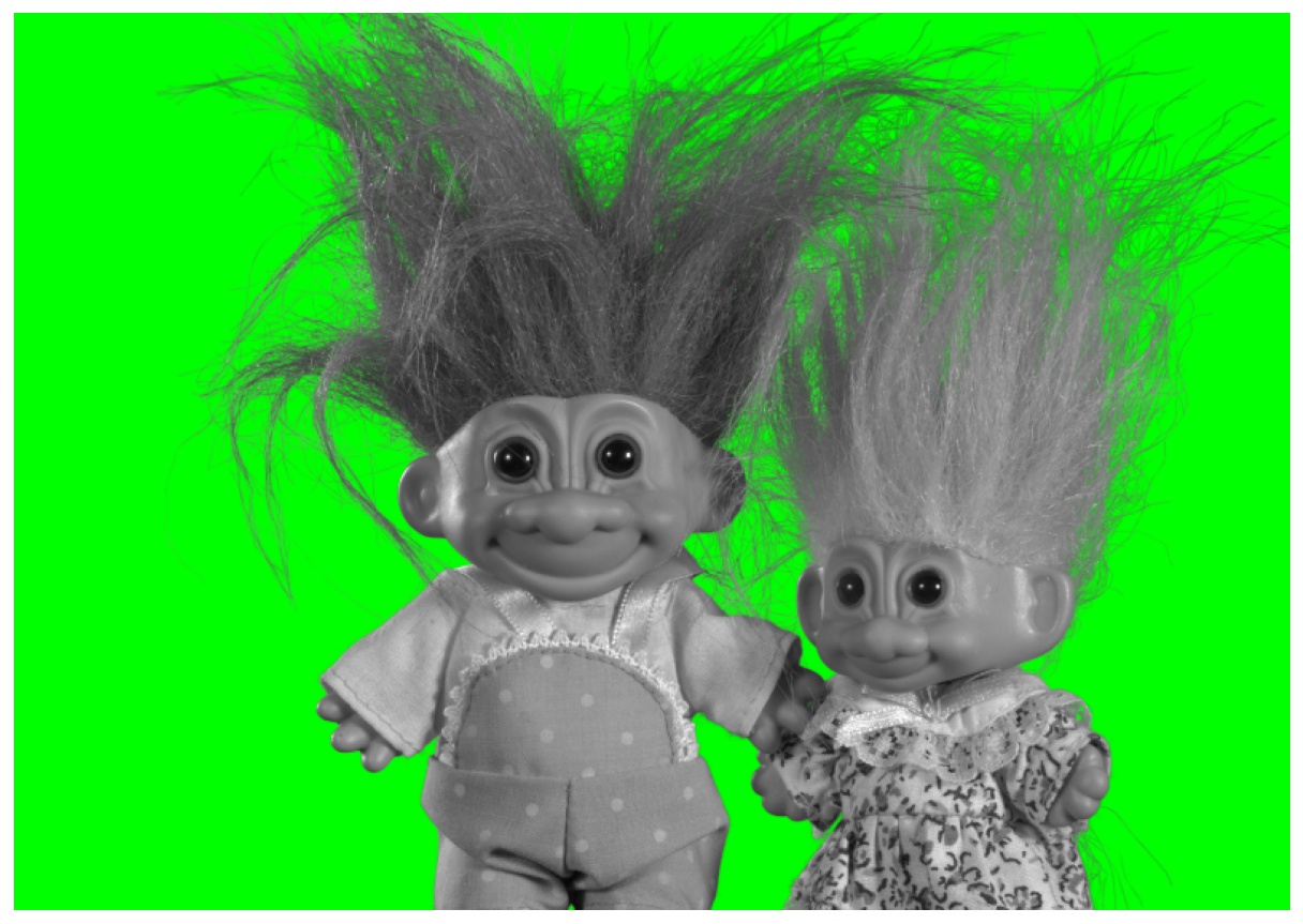
We create a gray version of the image with a green background as follows:
n_rows = I.shape[0]                              # number of rows in I
n_cols = I.shape[1]                              # number of columns in I
n_pixels = n_rows * n_cols                       # number of pixels in I
I = np.reshape(I, (n_pixels, 3))
I[:, 0] = I[:, 1]                                # red = green
I[:, 2] = I[:, 1]                                # blue = green
alpha_ex = np.reshape(alpha_ex, (n_pixels, 1))
G_B = 1                                          # green screen value
I = alpha_ex * I + (1 - alpha_ex) * [0, G_B, 0]  # replace background with green screen
I = np.reshape(I, (n_rows, n_cols, 3))
plt.imshow(I), plt.axis('off')                   # plot I
plt.show();
Let's extract the RGB components of \(I\):
R_I = I[:, :, 0]  # red component of I
G_I = I[:, :, 1]  # green component of I
B_I = I[:, :, 2]  # blue component of I
Let's compute the matte \(\alpha\):
alpha = (R_I - (G_I - G_B))/G_B                  # compute alpha with formula
plt.imshow(alpha, cmap='gray'), plt.axis('off')  # plot alpha
plt.show();

The relative error between our matte and the "exact" one is around machine precision:
alpha = np.reshape(alpha, (n_pixels, 1))
error = np.linalg.norm(alpha - alpha_ex)/np.linalg.norm(alpha_ex)
print(f'Error (alpha): {error:.2e}')
Error (alpha): 3.63e-17
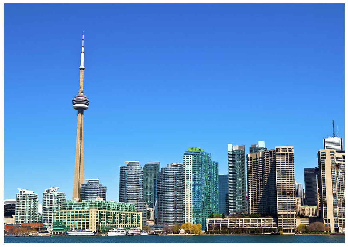
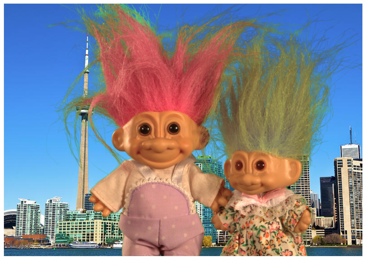
We're going to replace the green screen with the following image of Toronto's skyline:
K = cv2.imread('toronto.jpg')                # load image (BGR format)
K = cv2.cvtColor(K, cv2.COLOR_BGR2RGB)/255   # convert to RGB and normalize
K = K[:n_rows, :n_cols, :]                   # adjust size of K to size of I
plt.imshow(K), plt.axis('off')               # plot K
plt.show();
K = np.reshape(K, (n_pixels, 3))
Let's now replace the green screen with the image \(K\):
R_I = np.reshape(R_I, (n_pixels, 1))
J = np.tile(R_I, 3) + (1 - alpha) * K   # new image J with different background K
J = np.reshape(J, (n_rows, n_cols, 3))
plt.imshow(J), plt.axis('off')          # plot J
plt.show();
The result is flawless—it is not surprising that science fiction movies use green screens particularly well since many foreground objects are neutrally colored spacecraft.
Other exact solutions
Smith and Blinn [1] found an exact solution of the matting equation for foreground images \(F\) that verify $$ \mathrm{B}_F = a_0 + a_1\mathrm{G}_F, $$ for some coefficients \(a_0\) and \(a_1\). We present here a slightly more general solution for foreground images \(F\) that satisfy $$ \mathrm{B}_F = a_0 + a_1\mathrm{G}_F + a_2\mathrm{R}_F. $$ Using this relationship, we obtain the following system of equations, $$ \begin{bmatrix}\mathrm{R}_I\\\mathrm{G}_I\\\mathrm{B}_I\end{bmatrix} = \alpha\begin{bmatrix}\mathrm{R}_F\\\displaystyle\frac{\mathrm{B}_F - a_0 - a_2\mathrm{R}_F}{a_1}\\\mathrm{B}_F\end{bmatrix} + (1-\alpha)\begin{bmatrix}0\\\mathrm{G}_B\\0\end{bmatrix}. $$ Here, we have three variables \((\mathrm{R}_F,\mathrm{B}_F,\alpha)\). The three equations read $$ \left\{ \begin{array}{ll} \mathrm{R}_I = \alpha\mathrm{R}_F, \\ \mathrm{G}_I = \alpha\displaystyle\frac{\mathrm{B}_F - a_0 - a_2\mathrm{R}_F}{a_1} + (1-\alpha)\mathrm{G}_B, \\ \mathrm{B}_I = \alpha\mathrm{B}_F. \end{array} \right. $$ The first and third equations lead to $$ \alpha\mathrm{R}_F = \mathrm{R}_I, \quad \alpha\mathrm{B}_F = \mathrm{B}_I,$$ while the second equation gives \(\mathrm{G}_I = (\mathrm{B}_I - a_0\alpha - a_2\mathrm{R}_I)/a_1 + (1-\alpha)\mathrm{G}_B\), that is, $$ \alpha = \frac{\mathrm{B}_I - a_1(\mathrm{G}_I - \mathrm{G}_B) - a_2\mathrm{R}_I}{a_0 + a_1\mathrm{G}_B}. $$ Again, to obtain a new image \(J\) with a different background \(K\), one can simply compute $$ J = \alpha F +(1-\alpha)K, $$ that is, $$ \begin{align} \begin{bmatrix}\mathrm{R}_J\\\mathrm{G}_J\\\mathrm{B}_J\end{bmatrix} = \alpha\begin{bmatrix}\mathrm{R}_F\\\displaystyle\frac{\mathrm{B}_F - a_0 - a_2\mathrm{R}_F}{a_1}\\\mathrm{B}_F\end{bmatrix} + (1-\alpha)\begin{bmatrix}\mathrm{R}_K\\\mathrm{G}_K\\\mathrm{B}_K\end{bmatrix} = \begin{bmatrix}\mathrm{R}_I\\\displaystyle\frac{\mathrm{B}_I - a_0\alpha - a_2\mathrm{R}_I}{a_1}\\\mathrm{B}_I\end{bmatrix} +(1-\alpha)\begin{bmatrix}\mathrm{R}_K\\\mathrm{G}_K\\\mathrm{B}_K\end{bmatrix}. \end{align} $$
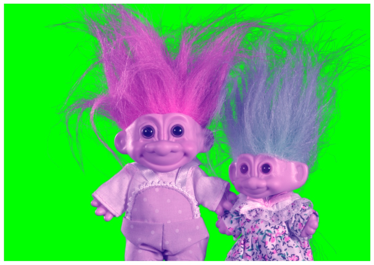
Let's create a version of the previous image that verifies a relationship of the form \(\mathrm{B}_F = a_0 + a_1\mathrm{G}_F + a_2\mathrm{R}_F\) with \(a_0=0.4\), \(a_1=0.3\) and \(a_2=0.3\):
I = cv2.imread('GT04.png')                       # load image I (BGR format)
I = cv2.cvtColor(I, cv2.COLOR_BGR2RGB)/255       # convert to RGB and normalize
I = np.reshape(I, (n_pixels, 3))
a_0 = 0.4                                        # coefficient a_0
a_1 = 0.3                                        # coefficient a_1
a_2 = 0.3                                        # coefficient a_2
I[:, 2] = a_0 + a_1*I[:, 1] + a_2*I[:, 0]        # blue = a_0 + a_1*green + a_2*red
I = alpha_ex * I + (1 - alpha_ex) * [0, G_B, 0]  # replace background with green screen
I = np.reshape(I, (n_rows, n_cols, 3))
plt.imshow(I), plt.axis('off')                   # plot I
plt.show();
Let's extract the RGB components of \(I\):
R_I = I[:, :, 0]  # red component of I
G_I = I[:, :, 1]  # green component of I
B_I = I[:, :, 2]  # blue component of I
Let's compute \(\alpha\):
alpha = (B_I - a_1*(G_I - G_B) - a_2*R_I)/(a_0 + a_1*G_B)  # compute alpha with formula
plt.imshow(alpha, cmap='gray'), plt.axis('off')            # plot alpha
plt.show();

Once again, the error is around machine precision:
alpha = np.reshape(alpha, (n_pixels, 1))
error = np.linalg.norm(alpha - alpha_ex)/np.linalg.norm(alpha_ex)  # relative error
print(f'Error (alpha): {error:.2e}')
Error (alpha): 1.46e-16
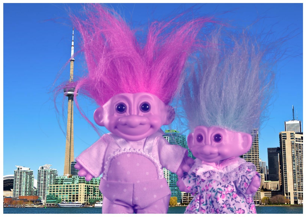
We can change the background as follows:
alpha = np.reshape(alpha, (n_pixels, 1))
R_I = np.reshape(R_I, (n_pixels, 1))
B_I = np.reshape(B_I, (n_pixels, 1))
J = np.concatenate((R_I, (B_I - a_0*alpha - a_2*R_I)/a_1, B_I), axis=1)  # new image J
J += (1 - alpha)*K
J = np.reshape(J, (n_rows, n_cols, 3))
plt.imshow(J), plt.axis('off')                                           # plot J
plt.show();
Extension and connection to Vlahos' formula
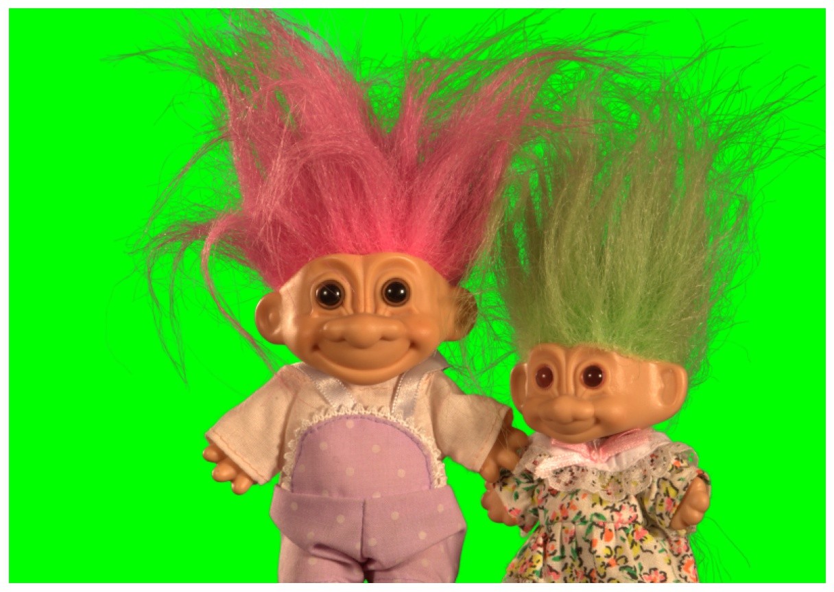
We've considered so far images whose RGB components verify specific relationships. For arbitrary color images, there is no exact formula for the matte \(\alpha\) and the foreground data \((\mathrm{R}_F,\mathrm{G}_F,\mathrm{B}_F)\). However, one may utilize the formula of the previous section as an approximation.
We show below an example with the color image we've been working with—this time, however, we use it as is with a green screen (i.e., we don't make it gray or purple-ish). We utilize the formula for the matte \(\alpha\) with \(a_0=0\), \(a_1=0.5\) and \(a_2=0\), which yields a relative error below \(8\%\). The resulting new image \(J\) with a different background \(K\) isn't perfect—let's emphasize that it was done with a very simple method that has an extremely low computational cost. Moreover, this image is particularly challenging because of the hair details and color. We provide below the full code in a single cell.
# Load the previous color image:
I = cv2.imread('GT04.png')
I = cv2.cvtColor(I, cv2.COLOR_BGR2RGB)/255
n_rows = I.shape[0]
n_cols = I.shape[1]
n_pixels = n_rows * n_cols
I = np.reshape(I, (n_pixels, 3))

# Load exact matte:
alpha_ex = cv2.imread('GT04_alpha.png', cv2.IMREAD_GRAYSCALE)/255
alpha_ex = np.reshape(alpha_ex, (n_pixels, 1))

# Generate a version with a green screen:
G_B = 1
I = alpha_ex * I + (1 - alpha_ex) * [0, G_B, 0]
I = np.reshape(I, (n_rows, n_cols, 3))
plt.imshow(I), plt.axis('off'), plt.show();

# RGB components:
R_I = I[:, :, 0]
G_I = I[:, :, 1]
B_I = I[:, :, 2]

# Coefficients:
a_0 = 0
a_1 = 0.5
a_2 = 0

# Compute alpha with formula:
alpha = (B_I - a_1*(G_I - G_B) - a_2*R_I)/(a_0 + a_1*G_B)
alpha[alpha < 0] = 0
alpha[alpha > 1] = 1
plt.imshow(alpha, cmap='gray'), plt.axis('off'), plt.show();

# Compute relative error with exact alpha:
alpha = np.reshape(alpha, (n_pixels, 1))
error = np.linalg.norm(alpha - alpha_ex)/np.linalg.norm(alpha_ex)
print(f'Error (alpha): {error:.2e}')

# Load background K:
K = cv2.imread('toronto.jpg')
K = cv2.cvtColor(K, cv2.COLOR_BGR2RGB)/255
K = K[:n_rows, :n_cols, :]
K = np.reshape(K, (n_pixels, 3))

# Compute new image J with background K:
alpha = np.reshape(alpha, (n_pixels, 1))
R_I = np.reshape(R_I, (n_pixels, 1))
B_I = np.reshape(B_I, (n_pixels, 1))
G_I = np.reshape(G_I, (n_pixels, 1))
tmp = np.minimum(G_I, (B_I - a_0*alpha - a_2*R_I)/a_1)
J = np.concatenate((R_I, tmp, B_I), axis=1) + (1 - alpha)*K
J[J < 0] = 0
J[J > 1] = 1
J = np.reshape(J, (n_rows, n_cols, 3))
plt.imshow(J), plt.axis('off'), plt.show();
Error (alpha): 7.58e-02
Let's make a few comments about the code. First, because the formula for the matte \(\alpha\) isn't exact here—it is merely an approximation—it may lead to values below \(0\) and above \(1\) for both \(\alpha\) and \(J\)—therefore, we clamped the values of \(\alpha\) and \(J\).
Second, the green component, which was given in the previous section by $$ \frac{\mathrm{B}_I - a_0\alpha - a_2\mathrm{R}_I}{a_1}, $$ has been replaced here with $$ \mathrm{min}\left(\mathrm{G}_I, \frac{\mathrm{B}_I - a_0\alpha - a_2\mathrm{R}_I}{a_1}\right). $$ This is inspired by Vlahos' work—Vlahos was an engineer who revolutionized the motion picture industry by introducing novel green screen techniques, essential to movies such as the Stars Wars trilogy and Titanic; he was awarded multiple Oscars and an Emmy Award for his contributions to the field.
In his first patent related to green screen technology [2], he claimed that for foreground images \(F\) that verify $$ \mathrm{G}_F \leq b_2\mathrm{B}_F, $$ the matte \(\alpha\) can be computed via the formula $$ \alpha = 1 - b_1(\mathrm{G}_I - b_2\mathrm{B}_I), $$ where \(b_1\) and \(b_2\) are tuning adjustment parameters. Once \(\alpha\) has been obtained by his formula, he proposed to compute the new image \(J\) with a different background \(K\) via $$ \begin{bmatrix}\mathrm{R}_J\\\mathrm{G}_J\\\mathrm{B}_J\end{bmatrix} = \begin{bmatrix}\mathrm{R}_I\\\mathrm{min}\left(\mathrm{G}_I, b_2\mathrm{B}_I\right)\\\mathrm{B}_I\end{bmatrix} +(1-\alpha)\begin{bmatrix}\mathrm{R}_K\\\mathrm{G}_K\\\mathrm{B}_K\end{bmatrix}. $$ In the code above, we selected \(a_0=a_2=0\), that is, we assumed that the foreground image \(F\) verifies $$ \mathrm{B}_F \approx a_1\mathrm{G}_F, $$ to some approximation. In that case, the formula for \(\alpha\) from the previous section simplifies to $$ \alpha = \frac{\mathrm{B}_I - a_1(\mathrm{G}_I - \mathrm{G}_B)}{a_1\mathrm{G}_B} = 1 - \frac{1}{\mathrm{G}_B}\left(\mathrm{G}_I - \frac{\mathrm{B}_I}{a_1}\right), $$ and the green component is given by $$ \begin{bmatrix}\mathrm{R}_J\\\mathrm{G}_J\\\mathrm{B}_J\end{bmatrix} = \begin{bmatrix}\mathrm{R}_I\\\displaystyle\frac{\mathrm{B}_I}{a_1}\\\mathrm{B}_I\end{bmatrix} +(1-\alpha)\begin{bmatrix}\mathrm{R}_K\\\mathrm{G}_K\\\mathrm{B}_K\end{bmatrix}. $$ This is exactly Vlahos' process provided that \(b_1=1/\mathrm{G}_B\), \(b_2=1/a_1\) and that we replace the green component with $$ \mathrm{min}\left(\mathrm{G}_I, \frac{\mathrm{B}_I}{a_1}\right), $$ which is precisely what we did.
Conclusion
Image matting is the process of recovering the matte \(\alpha\) and the foreground and background images \(F\) and \(B\) from an input image \(I\). This is an undetermined problem, which does not have exact solutions in general. When using a green screen, the problem becomes simpler and there are exact solutions in certain cases—for example when the foreground image \(F\) is gray.
For arbitrary color images, there exist simple green screen algorithms that lead to reasonably good numerical results—we've reviewed one of them, operating in RGB space.
In future blog posts, we'll talk about matting techniques without a green screen based on the Laplacian and deep neural networks, as well as video matting.
References
[1] A. R. Smith and J. F. Blinn, Blue screen matting, in Proceedings of the 23rd Annual Conference on Computer Graphics and Interactive Techniques, SIGGRAPH ’96, New York, NY, USA, 1996, Association for Computing Machinery, pp. 259–268.
[2] P. Vlahos, Electronic Composite Photography, U.S. Patent 3595987A, 1971.