November 28, 2020
In this post, I talk about quantum computing for solving nonlinear ordinary differential equations (ODEs). In a recent paper, Michael Lubasch and his colleagues proposed an algorithm to solve such equations using a combination of classical and quantum computers.
The main ideas are:
- reformulate the problem as an optimization one;
- use hybrid systems of quantum and classical computers to solve it.
The cost function and its gradient are typically evaluated on a quantum computer, while the higher-level iterative algorithm is performed on a classical computer.
Setup
The authors consider, as an example, the following nonlinear Schrödinger ODE eigenvalue problem, $$ \left[-\frac{1}{2}\frac{d^2}{dx^2} + V(x) + g\vert f(x)\vert^2\right]f(x) = \lambda f(x), $$ for \(x\in[a,b]\), and with \(f(a)=f(b)\) and \(\int_a^b\vert f(x)\vert^2dx=1\). They are only interested in the ground state of the problem, i.e., the function \(f\) that corresponds to the minimum eigenvalue \(\lambda_{\min}\). The nonlinear ODE eigenvalue problem reduces to a nonlinear ODE, which can be solved on a classical computer with an iterative method such as Newton's method, combined with, e.g., finite differences or a spectral method.
Method
The idea in the paper is to, instead, write the problem as an optimization one. They use the fact that the ground state minimizes the following cost function, $$ \begin{align} J(f) = \int_a^b\bigg[&\frac{1}{2}\vert f'(x)\vert^2+V(x)\vert f(x)\vert^2 +\frac{g}{2}\vert f(x)\vert^4\bigg]dx. \end{align} $$ They discretize \(J\) with the trapezoidal rule and finite differences on a uniform grid \(x_k=a+k(b-a)/N\), \(0\leq k\leq N-1\). The cost function \(J\) becomes a function of the \(N\) scaled values \(\psi_k=\sqrt{(b-a)/N}f(x_k)\). Then, they encode the \(N=2^n\) amplitudes \(\psi_k\) in the normalized state $$ \vert\psi\rangle = \sum_{k=0}^{N-1}\psi_k\vert\mathrm{binary}(k)\rangle, $$ where \(\mathrm{binary}(k)\) denotes the binary representation of the integer \(k=\sum_{j=1}^nq_j2^{n-j}\). Note that the above representation uses \(n\) qubits and basis states \(\vert\boldsymbol{q}\rangle=\vert q_1\ldots q_n\rangle\).
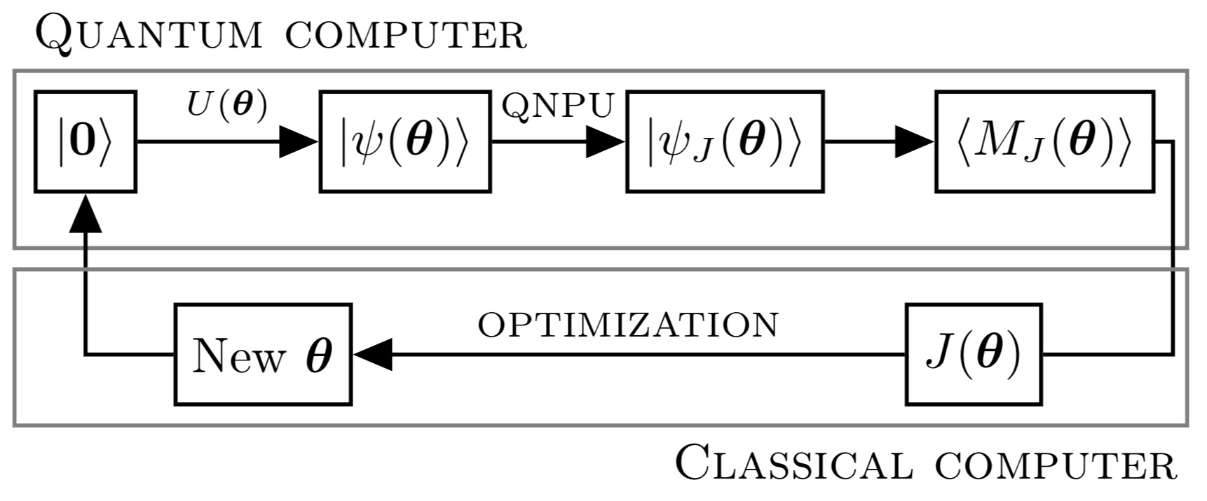
Their hybrid algorithm goes like this. First, the quantum register is put in a given state \(\vert\psi(\boldsymbol{\theta})\rangle=U(\boldsymbol{\theta})\vert\boldsymbol{0}\rangle\) via a quantum circuit \(U(\boldsymbol{\theta})\) of depth \(d=\mathcal{O}(\mathrm{poly}(n))\), such that their quantum ansatz requires \(\mathcal{O}(nd)=\mathcal{O}(\mathrm{poly}(n))\) parameters, exponentially fewer parameters than classical schemes—this is an example of quantum supremacy.
Second, a quantum nonlinear processing unit (QNPU) transforms the state \(\vert\psi(\boldsymbol{\theta})\rangle\) into a state \(\vert\psi_J(\boldsymbol{\theta})\rangle\) for which it is possible to measure a quantity \(\langle M_J(\boldsymbol{\theta})\rangle\) that is directly proportional to the cost function \(J(\boldsymbol{\theta})\).
Third, the evaluation of \(J(\boldsymbol{\theta})\) and the optimization over the parameters \(\boldsymbol{\theta}\) are carried out on a classical computer.
Theoretical justification
The quantum ansatz is based on matrix product states (MPS); for details, see, e.g., this. The key feature is that any state \(\psi\) can be written as $$ \vert\psi\rangle = \sum_{q_1,\ldots,q_n\in\{0,1\}}\mathrm{tr}\left[A^{(1)}_{q_1}\ldots A^{(n)}_{q_n}\right]\vert q_1\ldots q_n\rangle, $$ where \(A^{(k)}_0\) and \(A^{(k)}_1\) are \(D_k\times D_{k+1}\) matrices, for sufficiently large \(D_1,\ldots,D_{n+1}\). The bond dimension of such a representation is \(\chi=\max_{1\leq k\leq n+1} D_k\) and, in general, \(\chi=\mathcal{O}(\mathrm{exp}(n))\). States are referred to as MPS when \(\chi\) is not too big, typically when \(\chi=\mathcal{O}(\mathrm{poly}(n))\). Note that MPS require \(\mathcal{O}(n\chi^2)=\mathcal{O}(\mathrm{poly}(n))\) parameters (\(n\) matrices of size at most \(\chi\)).
The power of their quantum ansatz is that it contains all MPS with bond dimension \(\chi=\mathcal{O}(\mathrm{poly}(n))\). Since Chebyshev polynomials can be approximated exponentially well by MPS, MPS with such a \(\chi\) contain all polynomials of degree up to \(\mathcal{O}(\mathrm{exp}(\chi))=\mathcal{O}(N)\), as shown by Khoromskij here.
Classical MPS versus quantum ansatz
One could use a classical MPS-based method for a fairer comparison. To show the advantage of their quantum ansatz over classical MPS, they consider potentials of the form $$ V(x) = s_1\sin(\kappa_1 x) + s_2\sin(\kappa_2 x), $$ with \(\kappa_2=2\kappa_1/(1+\sqrt{5})\), and for various values of \(s_1/s_2\) and \(\kappa_1\). They show, both theoretically and numerically, that, in the \(s_1/s_2\approx1\) regime, the number of parameters for classical MPS scales like \(\mathcal{O}(\mathrm{poly}(\kappa_1))\), while it scales like \(\mathcal{O}(\log\kappa_1)\) for their quantum ansatz—quantum supremacy is achieved once again.
In the next and final episode of my series on quantum computing, I will talk about quantum computing for supervised learning.
Blog posts about quantum computing
- 2020 Quantum computing 4
- 2020 Quantum computing 3
- 2020 Quantum computing 2
- 2020 Quantum computing 1