December 6, 2020
In this post, I talk about quantum computing for supervised learning. Marcello Benedetti and his colleagues wrote a very nice review last year, which I highly recommend.
The main ideas are similar to those described in my previous post about quantum computing for ODEs:
- reformulate the problem as an optimization one;
- use hybrid systems of quantum and classical computers to solve it.
Setup
The core idea in supervised learning goes like this. We consider data \(\mathcal{X}\subseteq\mathbb{R}^d\), labels \(\mathcal{Y}\subseteq\mathbb{R}\) and a classifier \(f:\mathcal{X}\mapsto\mathcal{Y}\). We want to approximate \(f\) by \(\widehat{f}\) using \(n\) labeled data \((\boldsymbol{x}_1,y_1),\ldots,(\boldsymbol{x}_n,y_n)\in\mathcal{X}\times\mathcal{Y}\). The approximate classifier \(\widehat{f}\) is often parametrized by a vector of parameters \(\boldsymbol{\theta}\), and the training process consists in minimizing some cost function \(J(\boldsymbol{\theta})\).
They review two methods for quantum supervised machine learning, quantum kernel estimator (QKE) and variational quantum model (VQM). In both methods, the training set is mapped to feature space with a used-defined map \(\phi\) during the pre-processing stage.
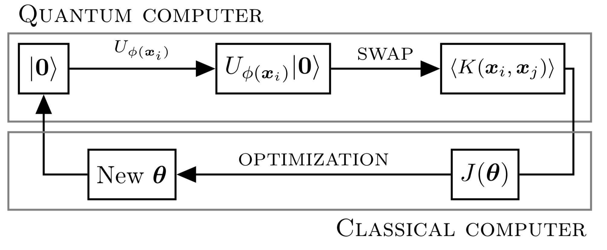
Method 1 (QKE)
First, the data \(\phi(\boldsymbol{x}_i)\) is encoded in a quantum circuit by applying some operator \(U_{\phi(\boldsymbol{x}_i)}\).
Second, a SWAP test is used to evaluate the kernel.
Third, the evaluation of \(J(\boldsymbol{\theta})\) and the optimization over the parameters \(\boldsymbol{\theta}\) are carried out on a classical computer. A typical example of such a \(J(\boldsymbol{\theta})\) would be the following quantum support-vector machines cost function, $$ J(\boldsymbol{\theta}) = \frac{1}{2}\sum_{i=1}^n\sum_{j=1}^n\theta_i\theta_jy_iy_j\langle K(\boldsymbol{x}_j,\boldsymbol{x}_i)\rangle-\sum_{i=1}^n\theta_i. $$
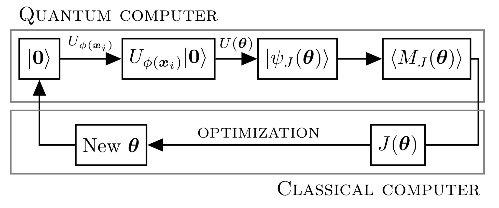
Method 2 (VQM)
The first step is the same as in QKE.
Second, a variational circuit \(U(\boldsymbol{\theta})\) implements the forecasting model. This yields state \(\vert\psi_J(\boldsymbol{\theta})\rangle\) for which it is possible to measure a quantity \(\langle M_J(\boldsymbol{\theta})\rangle\) that is directly related to the forecast.
Third, the evaluation of both the forecast \(\widehat{f}(\boldsymbol{x}_i;\langle M_J(\boldsymbol{\theta})\rangle)\) and \(J(\boldsymbol{\theta})\), which measures the forecasting error, as well as the optimization over \(\boldsymbol{\theta}\) are carried out on a classical computer. An example of a cost function \(J(\boldsymbol{\theta})\) would be $$ J(\boldsymbol{\theta}) = \frac{1}{n}\sum_{i=1}^n\left(\widehat{f}(\boldsymbol{x}_i;\langle M_J(\boldsymbol{\theta})\rangle)-y_i\right)^2. $$
Encoder circuit
The encoder circuit \(U_{\phi(\boldsymbol{x})}\) can be seen as an extra layer of feature-mapping, where the inner product defines a kernel $$ K(\boldsymbol{x}_i,\boldsymbol{x}_j)=\vert\langle\boldsymbol{0}\vert U^{*}_{\phi(\boldsymbol{x}_j)}U_{\phi(\boldsymbol{x}_i)}\vert\boldsymbol{0}\rangle\vert^2. $$ As I mentioned above, the SWAP test can then be used to estimate \(\langle K(\boldsymbol{x}_i,\boldsymbol{x}_j)\rangle\).
Variational circuit
In practice, the gate structure is fixed; only the gate parameters vary. A simple example of gate parametrization is given by $$ U(\boldsymbol{\theta}) = \prod_{\ell=1}^L\exp\left(-\frac{i}{2}\theta_\ell P_\ell\right), $$ where \(P_\ell\in\{I,Z,X,Y\}^{\otimes n}\) is a tensor of \(n\) Pauli matrices.
It is crucial to efficiently encode the variational circuit. A fixed gate structure allows for the number of gate parameters to grow polynomially in \(n\).
They emphasize on two key differences between variational circuits and neural networks. The first one is that quantum circuit operations are linear, as opposed to the nonlinear activation functions used in neural networks. The second one is that it is not possible to access the quantum state during the computation, which makes it hard to design a quantum analog of backpropagation.
Circuit learning
Circuit learning relies on standard optimization procedures, which are carried out on the classical computer. For simple gates such as the Pauli gates presented above, it is possible to derive a closed-form expression for the gradient with respect to \(\boldsymbol{\theta}\).
Blog posts about quantum computing
- 2020 Quantum computing 4
- 2020 Quantum computing 3
- 2020 Quantum computing 2
- 2020 Quantum computing 1