November 25, 2021
In this post, I talk about a new method for computing weakly singular and near-singular integrals that arise when solving the 3D Helmholtz equation with curved boundary elements.
Background on integral equations
The Helmholtz equation \(\Delta u + k^2u = 0\) in the presence of an obstacle may be rewritten as an integral equation on the obstacle's boundary via layer potentials. For example, the radiating solution to the Dirichlet problem \(\Delta u + k^2u = 0\) in \(\mathbb{R}^3\setminus\overline{\Omega}\) with \(u = u_D\) on the boundary \(\Gamma=\partial\Omega\), for some bounded \(\Omega\) whose complement is connected, can be obtained via the equation $$ \int_{\Gamma}G(\boldsymbol{x},\boldsymbol{y})\varphi(\boldsymbol{y})d\Gamma(\boldsymbol{y}) = u_D(\boldsymbol{x}), \quad \boldsymbol{x}\in\Gamma, $$ based on the single-layer potential; \(G\) is the Green's function of the Helmholtz equation in 3D, $$ G(\boldsymbol{x},\boldsymbol{y}) = \frac{1}{4\pi}\frac{e^{ik\vert\boldsymbol{x}-\boldsymbol{y}\vert}}{\vert\boldsymbol{x}-\boldsymbol{y}\vert}. $$ Once the equation is solved for \(\varphi\), which is unique if \(k^2\) is not an eigenvalue of \(-\Delta\) in \(\Omega\), the solution \(u\) may be represented by the left-hand side for all \(\boldsymbol{x}\in\mathbb{R}^3\setminus\Omega\). This technique is not limited to the Helmholtz equation, Maxwell's equations and elasticity problems can be reformulated as integral equations as well.
Challenges
From a numerical point of view, integral equations are particularly challenging for several reasons. First, when \(\boldsymbol{x}\) approaches \(\boldsymbol{y}\), the integral becomes singular and standard quadrature schemes fail to be accurate—analytic integration or carefully-derived quadrature formulas are, hence, required.
Second, the resulting linear systems after discretization are often dense. For large wavenumbers \(k\), only iterative methods can be used to solve them (with the help of specialized techniques to accelerate the matrix-vector products, such as the Fast Multipole Method or hierarchical matrices). In this respect, the use of higher-order numerical discretization schemes may be helpful in enlarging the interval of feasible wavenumbers.
Computing weakly singular integrals
When solving boundary integrals equations with curved boundary elements, one has to compute integrals of the form $$ I(\boldsymbol{x}_0) = \int_\mathcal{T}\frac{\varphi(F^{-1}(\boldsymbol{x}))}{\vert\boldsymbol{x} - \boldsymbol{x}_0\vert}dS(\boldsymbol{x}), $$ where \(\mathcal{T}\) is a curved triangle defined by a polynomial transformation \(F:\widehat{T}\to\mathcal{T}\) of degree \(q\geq1\) from some flat reference triangle \(\widehat{T}\), \(\boldsymbol{x}_0\) is a point on or close to \(\mathcal{T}\), and \(\varphi:\widehat{T}\to\mathbb{R}\) is a polynomial function of degree \(p\geq0\) (not necessarily equal to \(q\)). Our method is based on the computation of the preimage of the singularity on the reference element using Newton's method, singularity subtraction with high-order Taylor expansions, the continuation approach, and transplanted Gauss quadrature.
Step 1. We map \(\mathcal{T}\) back to \(\widehat{T}\), $$ I(\boldsymbol{x}_0) = \int_{\widehat{T}}\frac{\psi(\boldsymbol{\widehat{x}})}{\vert F(\boldsymbol{\widehat{x}}) - \boldsymbol{x}_0\vert}dS(\boldsymbol{\widehat{x}}), $$ where \(\psi(\boldsymbol{\widehat{x}})\) includes the Jacobian \(J\).
Step 2. We write $$ \boldsymbol{x}_0 = F(\boldsymbol{\widehat{x}}_0) + \boldsymbol{x}_0 - F(\boldsymbol{\widehat{x}}_0) $$ for some \(\boldsymbol{\widehat{x}}_0\in\widehat{T}\) such that its image \(F(\boldsymbol{\widehat{x}}_0)\in\mathcal{T}\) is the closest point to \(\boldsymbol{x}_0\) on \(\mathcal{T}\). In other words, we compute the preimage \(\boldsymbol{\widehat{x}}_0\) of the singularity or near-singularity. This can be done efficiently with Newton's method combined with a backtracking line search.
Step 3. We compute the singular or near-singular term using the first-order Taylor series of \(F(\boldsymbol{\widehat{x}}) - \boldsymbol{x}_0\) at \(\boldsymbol{\widehat{x}}_0\), $$ T_{-1}(\boldsymbol{\widehat{x}},h) = \frac{\psi(\boldsymbol{\widehat{x}}_0)}{\sqrt{\vert J(\boldsymbol{\widehat{x}}_0)(\boldsymbol{\widehat{x}} - \boldsymbol{\widehat{x}}_0)\vert^2 + h^2}}, $$ and add it to/subtract it from the original integral, $$ \begin{align} I(\boldsymbol{x}_0) = \, & \int_{\widehat{T}}T_{-1}(\boldsymbol{\widehat{x}},h)dS(\boldsymbol{\widehat{x}}) + \int_{\widehat{T}}\left[\frac{\psi(\boldsymbol{\widehat{x}})}{\vert F(\boldsymbol{\widehat{x}}) - \boldsymbol{x}_0\vert} - T_{-1}(\boldsymbol{\widehat{x}},h)\right]dS(\boldsymbol{\widehat{x}}). \end{align} $$ The first integral is singular or near-singular and will be computed in Steps 4–5. The second integral has a bounded integrand—it can be computed with Gauss quadrature on triangles. To render the integrand in the second integral smoother, which would accelerate convergence by quadrature, higher-order Taylor expansions may be added and subtracted.
Step 4. Let $$ I_{-1}(h) = \int_{\widehat{T}}T_{-1}(\boldsymbol{\widehat{x}},h)dS(\boldsymbol{\widehat{x}}). $$ The integrand is homogeneous in both \(\boldsymbol{\widehat{x}}\) and \(h\), and using the continuation approach, we reduce the 2D integral to a sum of three 1D integrals along the edges of \(\widehat{T}-\boldsymbol{\widehat{x}}_0\), $$ I_{-1}(h) = \psi(\boldsymbol{\widehat{x}}_0)\sum_{j=1}^3\widehat{s}_j\int_{\partial\widehat{T}_j - \boldsymbol{\widehat{x}}_0}f_{-1}(\boldsymbol{x},h)ds(\boldsymbol{\widehat{x}}), $$ where the \(\widehat{s}_j\)'s are the distances from the origin to the edges \(\partial\widehat{T}_j-\boldsymbol{\widehat{x}}_0\) of \(\widehat{T}-\boldsymbol{\widehat{x}}_0\), and $$ f_{-1}(\boldsymbol{\hat{x}},h) = \frac{\sqrt{\vert J(\boldsymbol{\widehat{x}}_0)\boldsymbol{\widehat{x}}\vert^2+h^2}-h}{\vert J(\boldsymbol{\widehat{x}}_0)\boldsymbol{\widehat{x}}\vert^2}. $$
Step 5. On the one hand, when the origin is far from all three edges (e.g., near the center of the triangle), each integrand is analytic and convergence with Gauss quadrature is exponential. On the other, when the origin lies on an edge, the corresponding integrand is singular—however, the distance \(\widehat{s}_j\) to that edge equals \(0\), the product “\(\widehat{s}_j\) times integral” is also \(0\), and the integral need not be computed. Issues arise when the origin is close to one of the edges—the integrand is analytic but near-singular, convergence with Gauss quadrature is exponential but slow. We circumvent the near-singularity issue by using transplanted Gauss quadrature.
Numerical experiments
Let \(\Omega\subset\mathbb{R}^3\) be a bounded domain whose complement is connected, let \(\Gamma\) be its boundary, and let \(k>0\). Given an incident wave \(u^i\), a solution to \(\Delta u + k^2u = 0\) in \(\mathbb{R}^3\), we look for the scattered field \(u^s\), a solution to \(\Delta u + k^2u = 0\) in \(\mathbb{R}^3\setminus\overline{\Omega}\), satisfying the Sommerfeld radiation condition and such that \(u^i(\boldsymbol{x}) + u^s(\boldsymbol{x}) = 0\) on \(\Gamma=\partial\Omega\). As said above, this leads to $$ \frac{1}{4\pi}\int_{\Gamma}\frac{e^{ik\vert\boldsymbol{x}-\boldsymbol{y}\vert}}{\vert\boldsymbol{x}-\boldsymbol{y}\vert}\varphi(\boldsymbol{y})d\Gamma(\boldsymbol{y}) = -u^i(\boldsymbol{x}), $$ for \(\boldsymbol{x}\in\Gamma\). Once the equation is solved for \(\varphi\), the solution \(u^s\) for all \(x\in\mathbb{R}^3\setminus\Omega\) is given by $$ u^s(\boldsymbol{x}) = \frac{1}{4\pi}\int_{\Gamma}\frac{e^{ik\vert\boldsymbol{x}-\boldsymbol{y}\vert}}{\vert\boldsymbol{x}-\boldsymbol{y}\vert}\varphi(\boldsymbol{y})d\Gamma(\boldsymbol{y}). $$
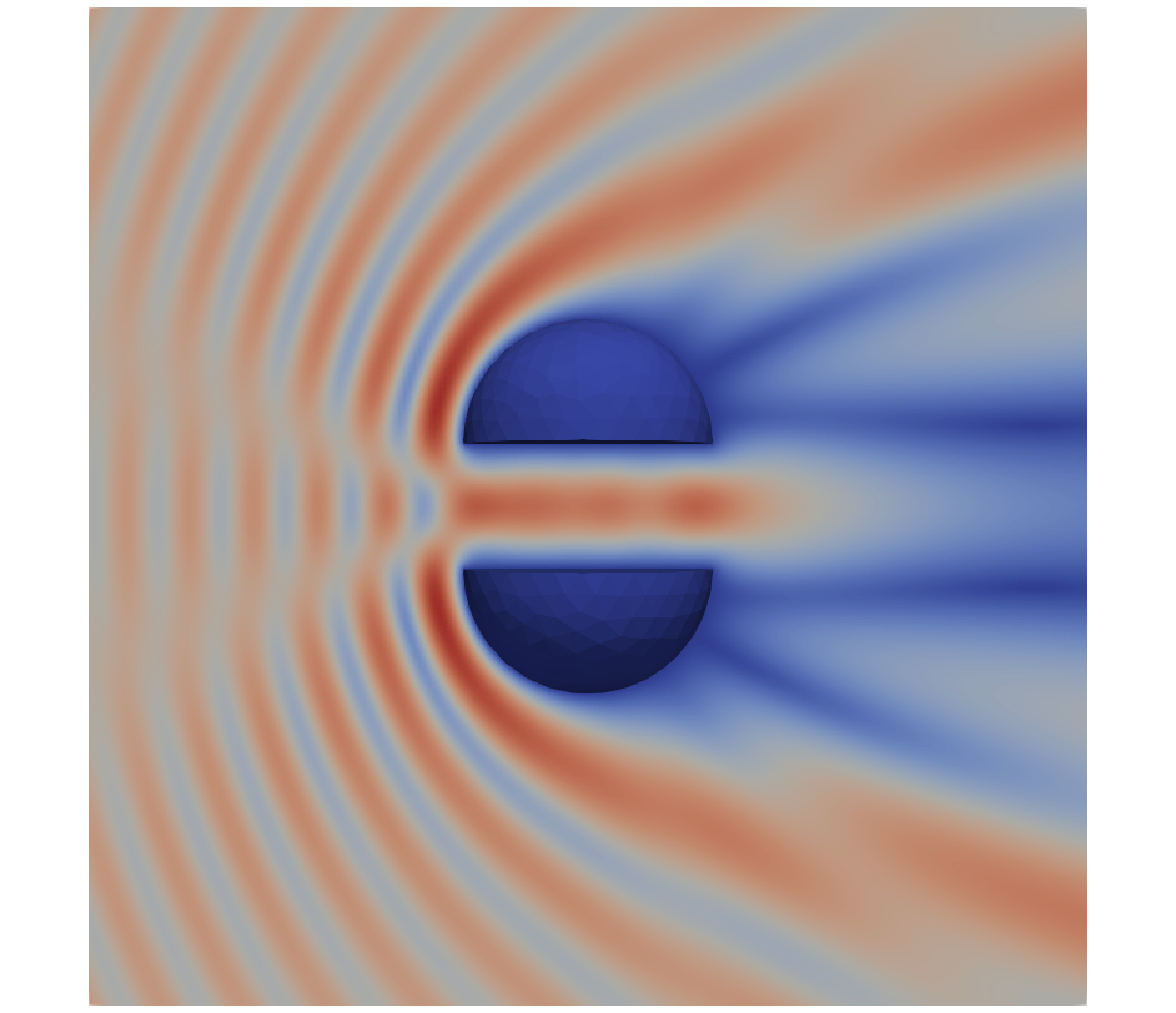
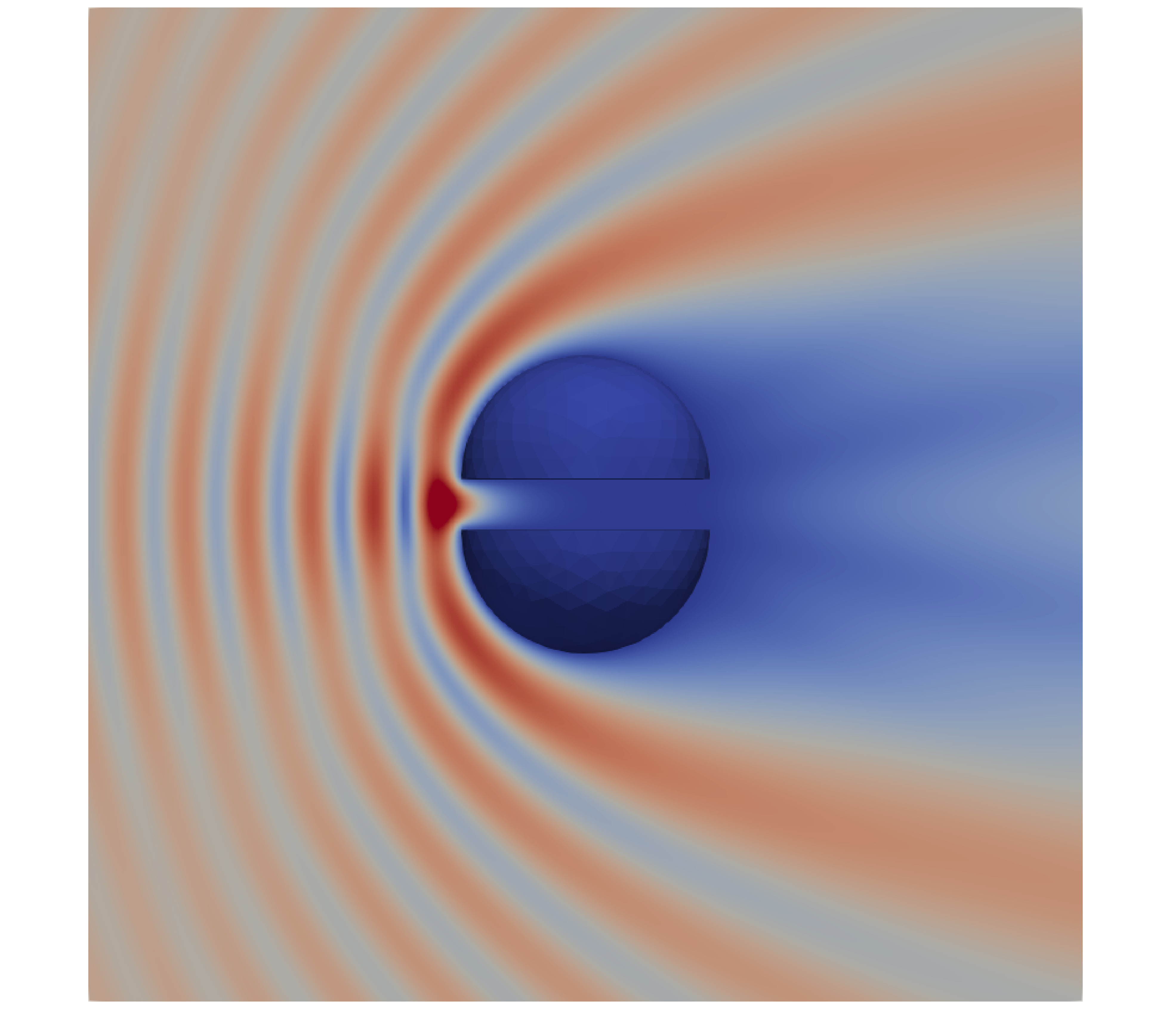
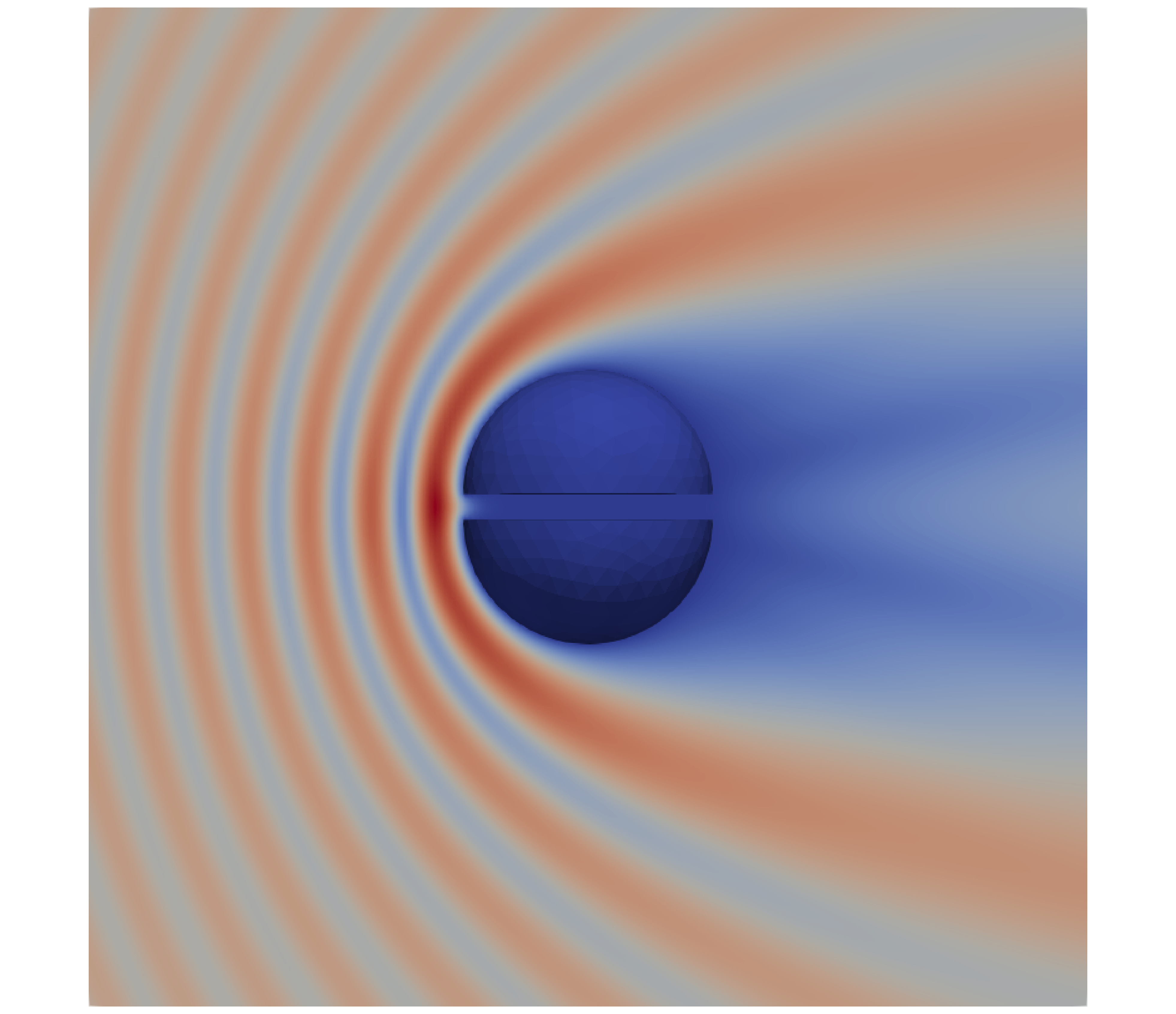
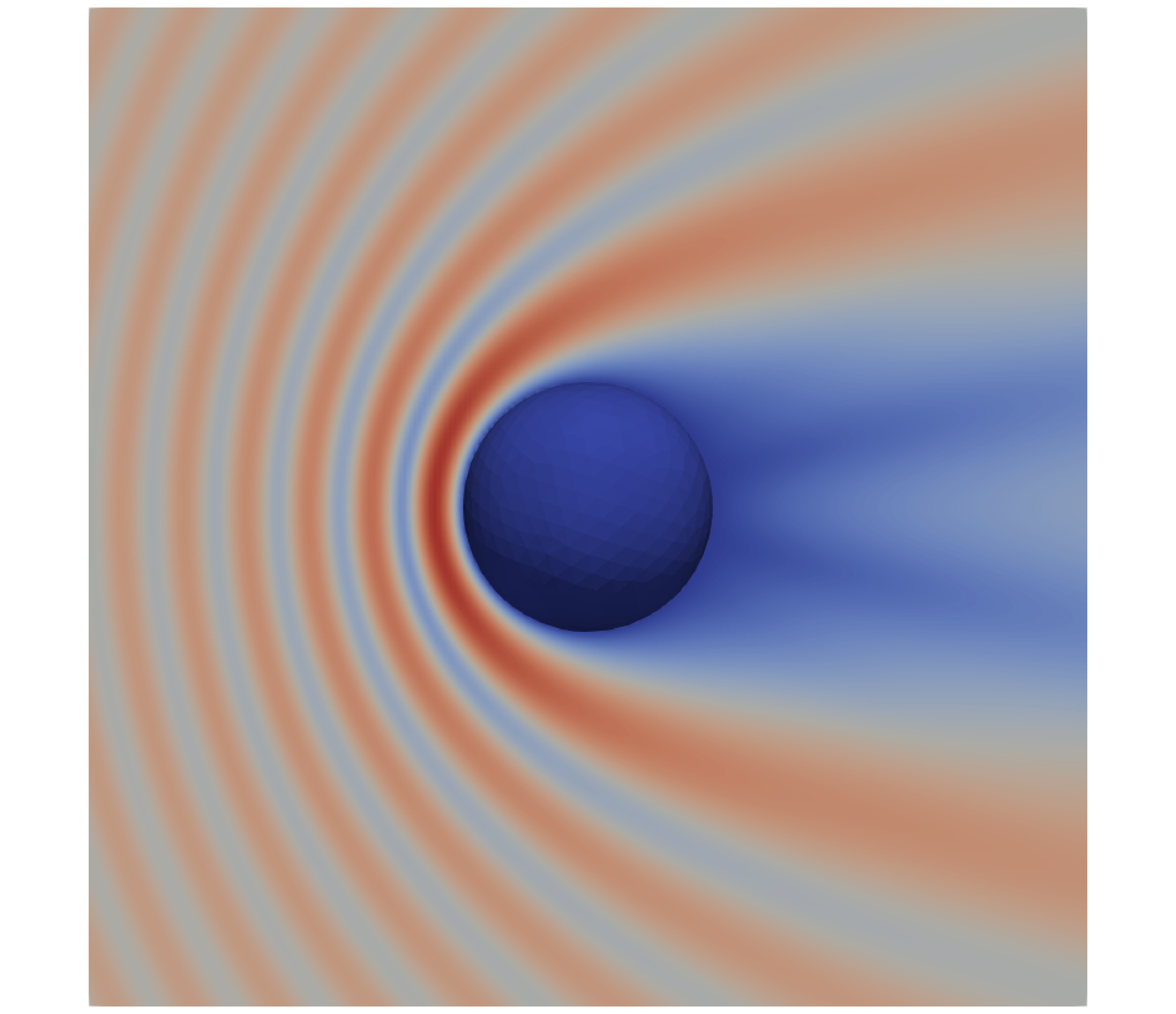
We discretize the integral equation using quadratic boundary elements together with our method for computing singular integrals. We take \(k=2\pi\) and consider the scattering of a plane wave \(u^i(r,\theta)=e^{ikr\cos\theta}\) by two half-spheres of radius \(1\) centered at \((0,0,\pm\delta)\) for small values of \(\delta\). For each of these values, we solve the equation and evaluate the total field \(u=u^i+u^s\) for a mesh size \(h\approx10^{-1}\), which guarantees about five digits of accuracy. We plot \(u\) below for \(\delta=0.5,0.2,0.1,0\). Let us emphasize that this numerical experiment is particularly challenging when \(\delta\ll h\). Standard methods like that of Sauter and Schwab fail to be accurate in this regime; our method produced accurate results for \(h\approx10^{-1}\) and \(\delta\) as small as \(5\times10^{-4}\). Check out our paper!