February 12, 2023
In this post, I talk about coupling the finite and boundary element methods for solving wave propagation problems in an inhomogeneous medium.
Acoustic waves in an inhomogeneous medium

We consider the following model with a total field \(u\) coupled with a scattered field \(w^s\): $$ \begin{align} & \Delta u + k^2nu = 0 \quad \text{in $B\setminus\overline{D}$}, \\[.4em] & u = 0 \quad \text{on $\partial D$}, \\[0.4em] & \Delta w^s + k^2w^s = 0 \quad \text{in $\mathbb{R}^2\setminus\overline{B}$}, \\[.4em] & \text{$w^s$ is radiating}, \\[0.4em] & \displaystyle w^s = u - u^i \;\,\text{and}\;\, \frac{\partial w^s}{\partial\nu} = \frac{\partial (u - u^i)}{\partial\nu} \quad \text{on $\partial B$}. \end{align} $$ The part of the domain where the refractive index \(n\neq1\) models an inhomogeneous medium. For the applications I am interested in, \(n\) is often a (smooth) random function.
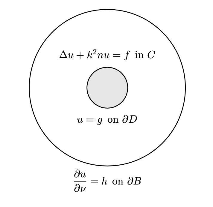
To solve this system, we must be able to solve interior problems of the form $$ \begin{align} & \Delta u + k^2nu = f \quad \text{in $B\setminus\overline{D}$}, \\[0.4em] & u = g \quad \text{on $\partial D$}, \\[0.4em] & \frac{\partial u}{\partial\nu} = h \quad \text{on $\partial B$}, \end{align} $$ with a fine element method, as well as exterior problems of the form $$ \begin{align} & \Delta w + k^2w = 0 \quad \text{in $\mathbb{R}^2\setminus\overline{B}$}, \\[0.4em] & w = g \quad \text{on $\partial B$}, \\[0.4em] & \text{$w$ is radiating}, \end{align} $$ with a boundary element method.
Interior problems & finite elements
Theory (disk)
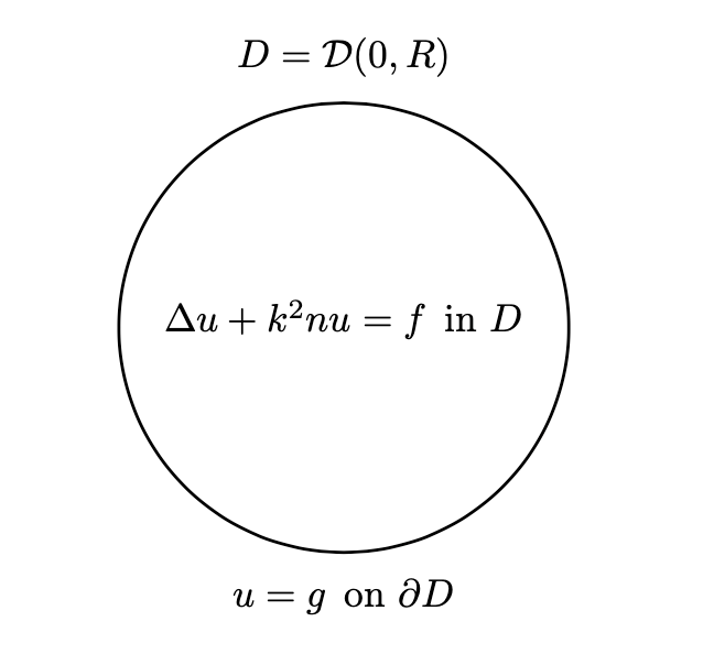
Let \(D=\mathcal{D}(0,R)\), the disk of radius \(R>0\) centered at the origin, and consider \begin{align*} & \Delta u + k^2nu = f \quad \text{in $D$}, \\[0.4em] & u = g \quad \text{on $\partial D$}, \end{align*} for some \(g\) such that \(\Delta g = 0\) in \(D\). Let us define \(\widetilde{u} = u - g\). Then, $$ \begin{align} & \Delta \widetilde{u} + k^2n\widetilde{u} = f - k^2ng \quad \text{in $D$}, \\[0.4em] & \widetilde{u} = 0 \quad \text{on $\partial D$}. \end{align} $$ The variational problem is to find \(\widetilde{u}\in H^1_0(D)\) such that $$ \int_D\left(-\nabla\widetilde{u}\nabla v + k^2n\widetilde{u}v\right) = \int_D (f - k^2ng)v, $$ for all \(v\in H^1_0(D)\), where $$ H^1_0(D) = \left\{v \in H^1(D) \,:\, v|_{\partial D} = 0\right\}. $$ Once the problem is solved for \(\widetilde{u}\), we recover \(u=\widetilde{u}+g\).
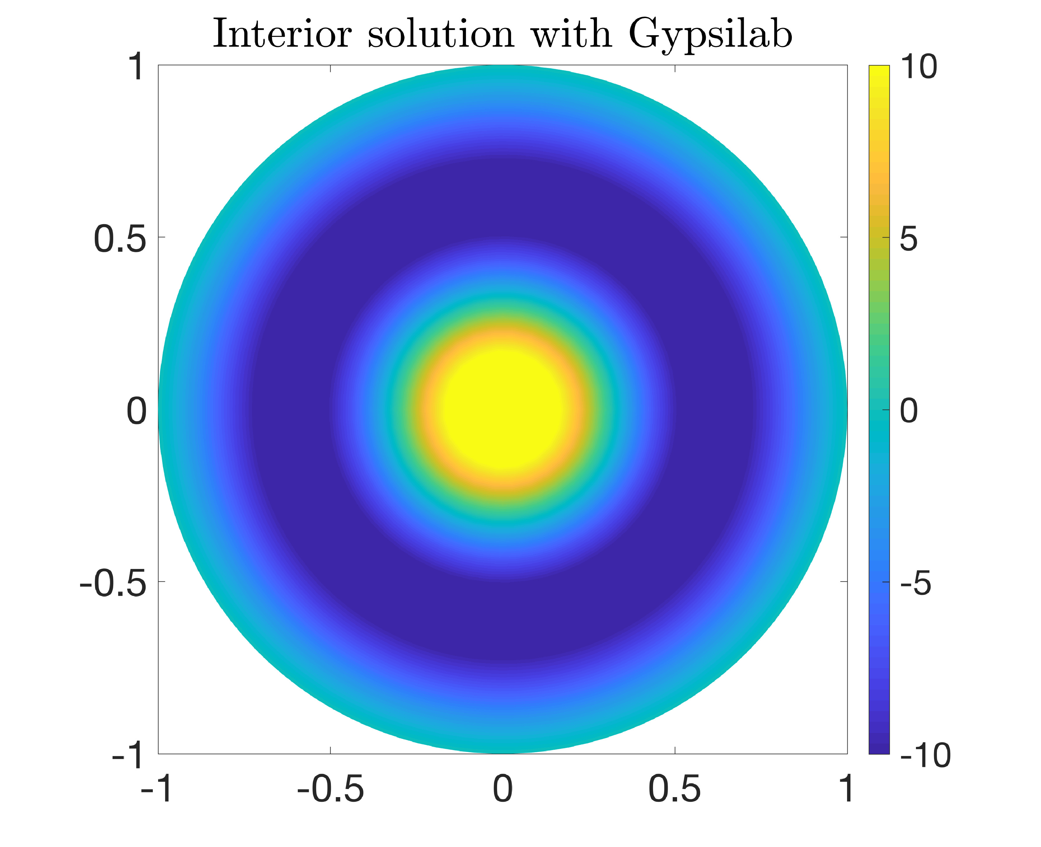
Experiment (disk)
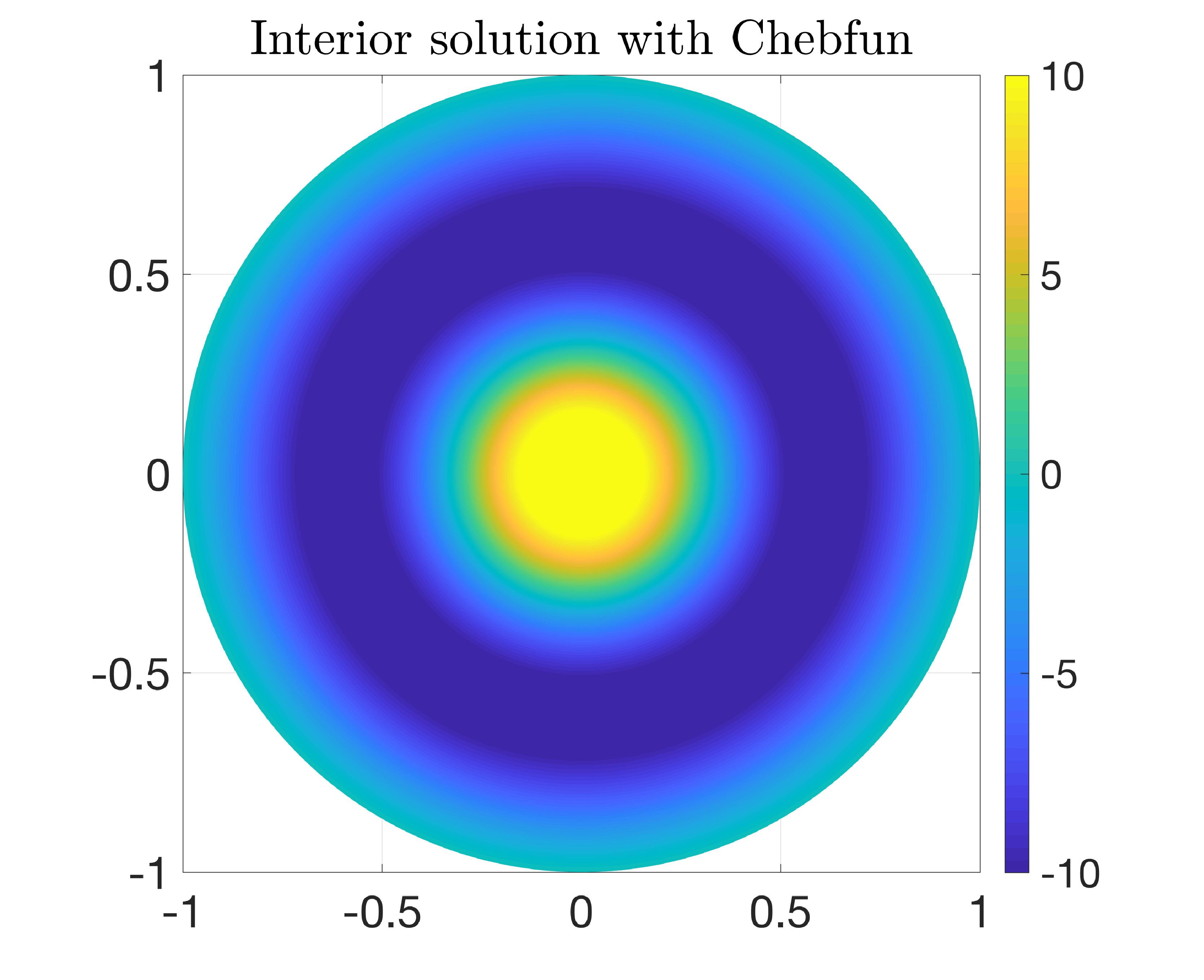
Let us take \(R=1\), \(k=2\pi\), and $$ n(x,y)=1, \quad f(x,y)=x^2, \quad g(x,y)=4. $$ Using the gypsilab toolbox, we may compute the solution as follows.
R = 1;
k = 2*pi;
n = @(X) 0*X(:, 1) + 1;
f = @(X) X(:, 1).^2;
g = @(X) 0*X(:, 1) + 4;
N = 1000;
mesh = mshDisk(N, R);
D = dom(mesh, 3);
V = fem(mesh, 'P1');
V = dirichlet(V, mesh.bnd);
L = -integral(D, grad(V), grad(V)) ...
+ k^2*integral(D, V, n, V);
F = integral(D, V, @(X) f(X) - k^2*n(X).*g(X));
u = L\F;
In Chebfun, we may use the diskfun.helmholtz code.
F = diskfun(@(x,y) f([x, y]) - k^2*g([x, y]));
BC = @(theta) 0*theta;
u = diskfun.helmholtz(F, k, BC, N);
Theory (annulus)
Let us now consider a harder problem. Let \(D=\mathcal{D}(0, R_1)\) and \(B=\mathcal{D}(0,R_2)\) for some \(R_2>R_1>0\). Define \(C=B\setminus\overline{D}\) and consider $$ \begin{align} & \Delta u + k^2nu = f \quad \text{in $C$}, \\[0.4em] & u = g \quad \text{on $\partial D$}, \\[0.4em] & \frac{\partial u}{\partial\nu} = h \quad \text{on $\partial B$}, \end{align} $$ for some \(g\) such that \(\Delta g = 0\) in \(C\) and \(\partial g/\partial\nu = 0\) on \(\partial B\). Let us define \(\widetilde{u} = u - g\). Then, $$ \begin{align} & \Delta \widetilde{u} + k^2n\widetilde{u} = f - k^2ng \quad \text{in $C$}, \\[0.4em] & \widetilde{u} = 0 \quad \text{on $\partial D$}, \\[0.4em] & \frac{\partial\widetilde{u}}{\partial\nu} = h \quad \text{on $\partial B$}. \end{align} $$ The problem is to find \(\widetilde{u}\in H^1_0(C)\) such that $$ \int_{C}\left(-\nabla\widetilde{u}\nabla v + k^2n\widetilde{u}v\right) = \int_{C} (f - k^2ng)v - \int_{\partial B}hv, $$ for all \(v\in H^1_0(C)\), where (slight abuse of notation) $$ H^1_0(C) = \left\{v \in H^1(C) \,:\, v|_{\partial D} = 0\right\}. $$ Once the problem is solved for \(\widetilde{u}\), we recover \(u=\widetilde{u}+g\).
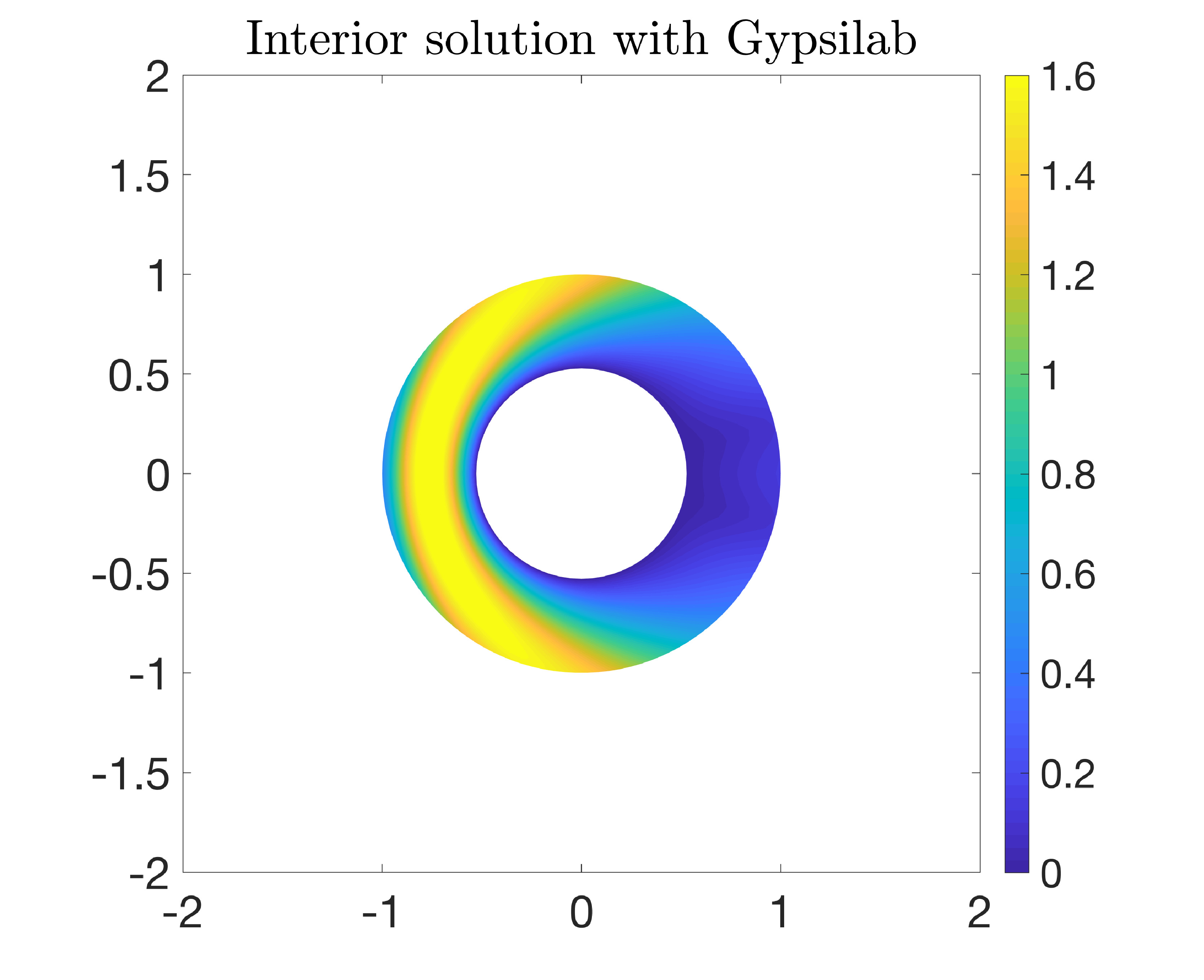
Experiment (annulus)
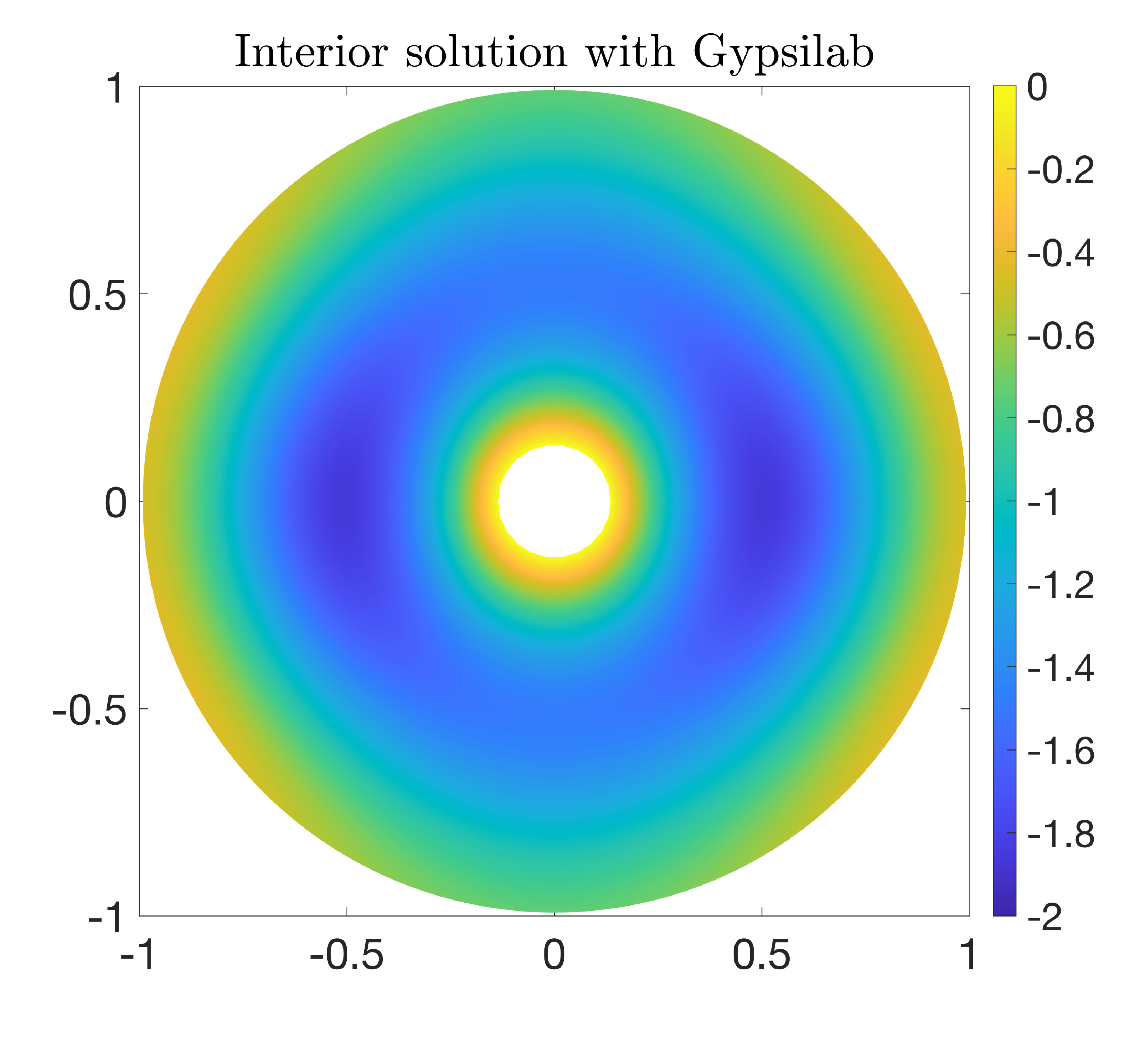
Let us take \(R_1=0.1\), \(R_2=1\), \(k=2\pi\), $$ n(x,y)=\cos(y), \quad f(x,y)=x^2, $$ and \(g(x,y) = h(x,y) = 1\).
R1 = 0.1;
R2 = 1;
k = 2*pi;
n = @(X) cos(X(:, 2));
f = @(X) X(:, 1).^2;
g = @(X) 0*X(:, 1) + 1;
h = @(X) 0*X(:, 1) + 1;
N = 2000;
mesh = mshAnnulus(N, R1, R2);
C = dom(mesh, 3);
[dD, dB] = bndAnnulus(mesh.bnd);
dB = dom(dB, 3);
V = fem(mesh, 'P1');
V = dirichlet(V, dD);
L = -integral(C, grad(V), grad(V)) ...
+ k^2*integral(C, V, n, V);
F = integral(C, V, @(X) f(X) - k^2*n(X).*g(X)) ...
- integral(dB, V, h);
u = L\F;
Exterior problems & boundary elements
Theory
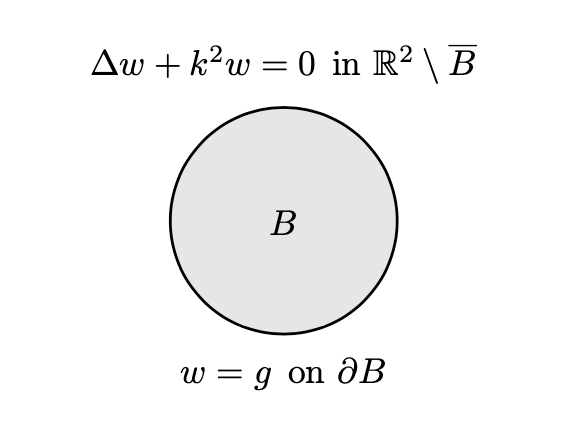
Let \(B=\mathcal{D}(0,R)\) and consider $$ \begin{align} & \Delta w + k^2w = 0 \quad \text{in $\mathbb{R}^2\setminus\overline{B}$}, \\[0.4em] & w = g \quad \text{on $\partial B$}, \quad \text{$w$ is radiating}, \end{align} $$ for some function \(g\). Let us look for \(w\) as a single-layer potential, $$ w(\boldsymbol{x}) = \int_{\partial B} G(\boldsymbol{x},\boldsymbol{y})\varphi(\boldsymbol{y})dS(\boldsymbol{y}) = (\mathcal{S}\varphi)(\boldsymbol{x}). $$ The problem is to find \(\varphi\in H^{-1/2}(\partial B)\) such that $$ \int_{\partial B}(\mathcal{S}\varphi)(\boldsymbol{x})\psi(\boldsymbol{x})dS(\boldsymbol{x}) = \int_{\partial B}g(\boldsymbol{x})\psi(\boldsymbol{x})dS(\boldsymbol{x}), $$ for all \(\psi\in H^{-1/2}(\partial B)\).
Experimemt
Let us take \(R=0.5\), \(k=2\pi\), and $$ g(x,y) = -e^{ikx}. $$
R = 0.5;
k = 2*pi;
g = @(X) -exp(1i*k*X(:,1));
G = @(X,Y) femGreenKernel(X, Y, '[H0(kr)]', k);
N = 100;
mesh = mshCircle(N, R);
dB = dom(mesh, 3);
W = fem(mesh, 'P1');
S = (1i/4)*integral(dB, dB, W, G, W);
S = S - 1/(2*pi)*regularize(dB, dB, W, ...
'[log(r)]', W);
F = integral(dB, W, g);
phi = S\F;
Finite-boundary element coupling
Theory
We now come back to the initial problem:
$$
\begin{align}
& \Delta u + k^2nu = 0 \quad \text{in $B\setminus\overline{D}$}, \\[.4em]
& u = 0 \quad \text{on $\partial D$}, \\[0.4em]
& \Delta w^s + k^2w^s = 0 \quad \text{in $\mathbb{R}^2\setminus\overline{B}$}, \\[.4em]
& \text{$w^s$ is radiating}, \\[0.4em]
& \displaystyle w^s = u - u^i \;\,\text{and}\;\, \frac{\partial w^s}{\partial\nu} = \frac{\partial (u - u^i)}{\partial\nu} \quad \text{on $\partial B$}.
\end{align}
$$
Let \(D=\mathcal{D}(0, R_1)\), \(B=\mathcal{D}(0,R_2)\) for some \(R_2>R_1>0\), and \(C=B\setminus\overline{D}\). Combining the theory of the previous sections for interior and exterior problems, we define a bilinear form \(A\) with entries
$$
\begin{pmatrix}
\displaystyle \int_{\partial B}(\mathcal{S}\varphi)\psi & \displaystyle -\int_{\partial B}u\psi \\[.4em]
\displaystyle \int_{\partial B}\left[\left(\mathcal{D}^* - \frac{\mathcal{I}}{2}\right)\varphi\right]v & \displaystyle \int_C\left(-\nabla u\nabla v + k^2nuv\right)
\end{pmatrix},
$$
while the linear form \(F\) has entries
$$
\begin{pmatrix}
\displaystyle -\int_{\partial B} u^i\psi \\[.4em]
\displaystyle -\int_{\partial B}\frac{\partial u^i}{\partial \nu}v
\end{pmatrix},
$$
for \(\varphi,\psi\in H^{-1/2}(\partial B)\) and \(u,v\in H^1_0(C)\). We may write the system as
$$
\left\{
\begin{array}{l}
A_{11}\varphi + A_{12} u = F_1, \\[.4em]
A_{21}\varphi + A_{22} u = F_2.
\end{array}
\right.
$$
This yields
$$
\left\{
\begin{array}{l}
-A_{21}A_{11}^{-1}A_{12}u + A_{22}u = F_2 - A_{21}A_{11}^{-1}F_1, \\[.4em]
\varphi = A_{11}^{-1}(F_1 - A_{12}u).
\end{array}
\right.
$$
We use GMRES for the first equation (mgcr in gypsilab).
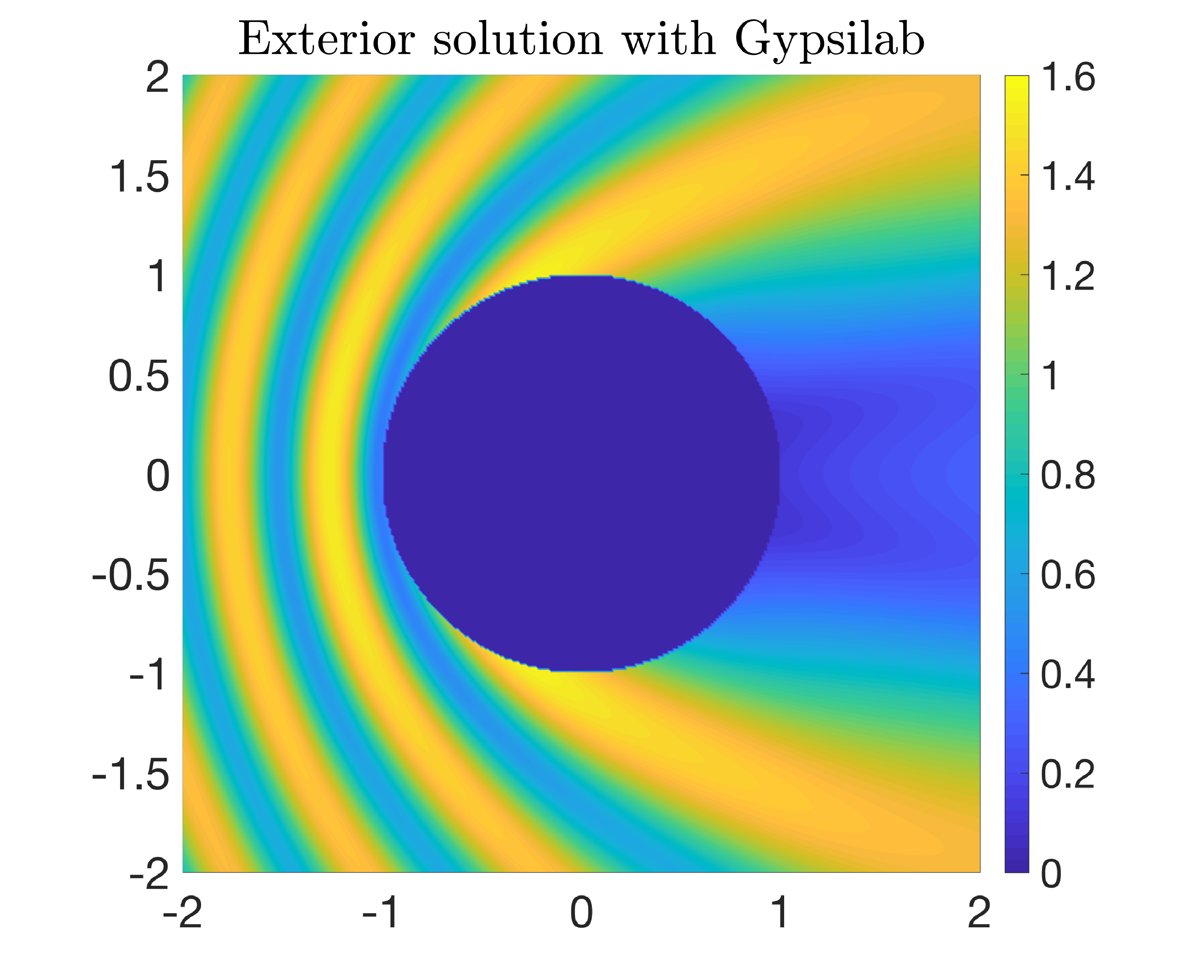
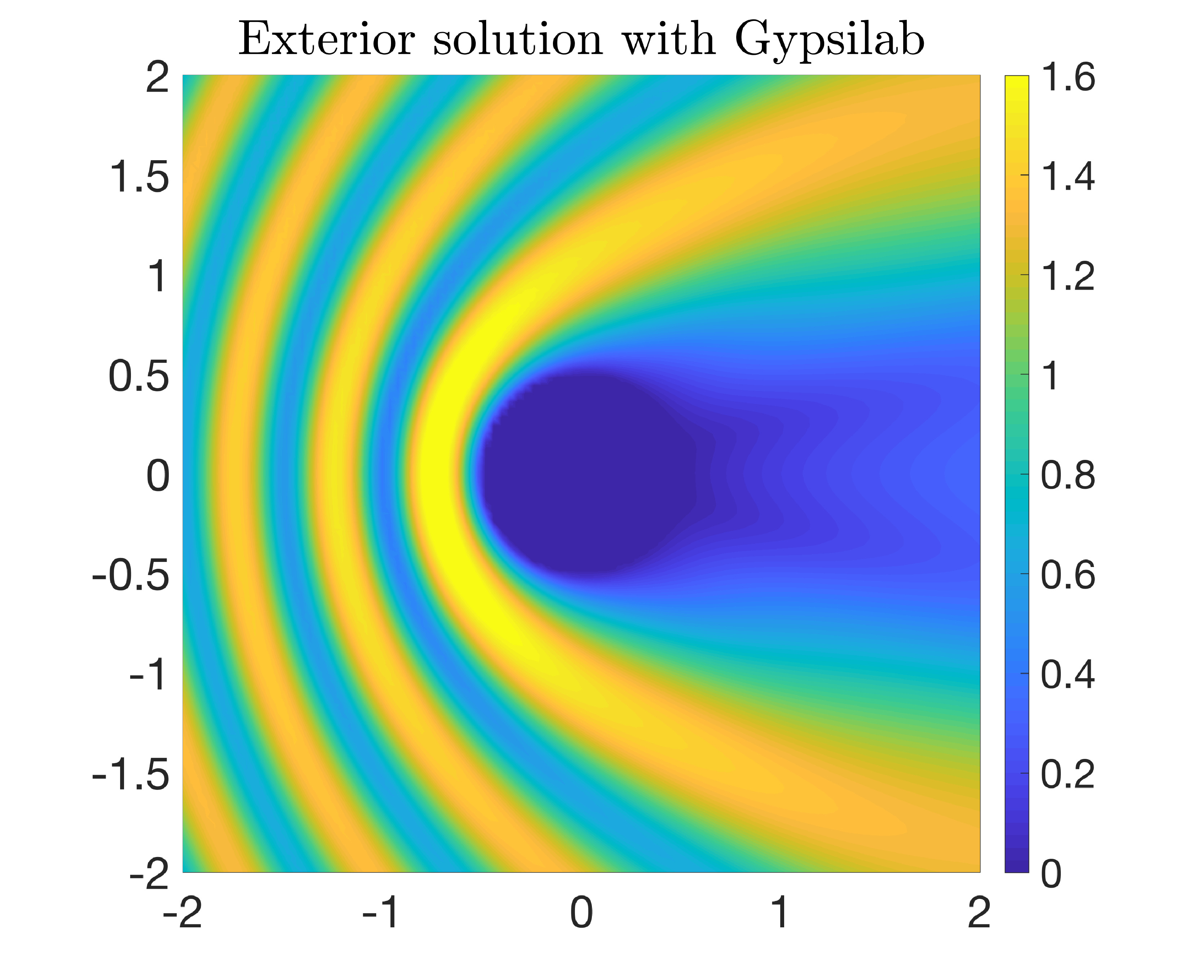
Experiment
Let us take \(R_1=0.5\), \(R_2=1\), \(k=2\pi\), and $$ u^i(x,y) = e^{ikx}, \quad n(x,y)=1. $$ Since we take \(n=1\) everywhere, we should recover the numerical solution of the previous section. The MATLAB code is a little bit more involved. We are going to break it down. We first set up the parameters.
R1 = 0.5;
R2 = 1;
k = 2*pi;
lambda = 2*pi/k;
ui = @(X) exp(1i*k*X(:, 1));
dui = @(X) 1i*k*X(:,1)/R2.*ui(X);
G = @(X,Y) femGreenKernel(X, Y, '[H0(kr)]', k);
dG{1} = @(X,Y) femGreenKernel(X, Y, ...
'grady[H0(kr)]1', k);
dG{2} = @(X,Y) femGreenKernel(X, Y, ...
'grady[H0(kr)]2', k);
dG{3} = @(X,Y) femGreenKernel(X, Y, ...
'grady[H0(kr)]3', k);
n = @(X) 0*X(:, 1) + 1;
We define the mesh and the finite/boundary elements.
N = 1000;
mesh = mshAnnulus(N, R1, R2);
C = dom(mesh, 3);
[dD, dB] = bndAnnulus(mesh.bnd);
V = fem(mesh, 'P1');
V = dirichlet(V, dD);
W = fem(dB, 'P1');
dB = dom(dB, 3);
This is the tricky part where we define the projection between finite and boundary elements, as well as the operators. (The negative sign in the double-layer variable D is to adjust the direction of the normal.)
[~, IW, IV] = intersect(W.unk, V.unk, 'rows');
P = sparse(IW, IV, 1, size(W.unk, 1), size(V.unk, 1));
L = -integral(C, grad(V), grad(V)) ...
+ k^2*integral(C, V, n, V);
S = (1i/4)*integral(dB, dB, W, G, W);
S = S - 1/(2*pi)*regularize(dB, dB, W, ...
'[log(r)]', W);
D = (1i/4)*integral(dB, dB, W, dG, ntimes(W));
D = D - 1/(2*pi)*regularize(dB, dB, W, ...
'grady[log(r)]', ntimes(W));
D = -D;
I = integral(dB, W, W);
We assemble the system and solve it.
A11 = S;
A21 = P'*(D.' - I/2);
A12 = -I*P;
A22 = L;
F1 = -integral(dB, W, ui);
F2 = -integral(dB, V, dui);
fun = @(V) -A21*(A11\(A12*V)) + A22*V;
u = mgcr(fun, F2 - A21*(A11\F1), [], 1e-3, 1000);
phi = A11\(F1 - A12*u);