May 19, 2020
One of the papers I wrote during my Ph.D. at Oxford with Niall Bootland was just accepted in Mathematics and Computers in Simulation. In this post, I review the main ideas of the paper.
Periodic stiff PDEs
We are interested in computing smooth solutions in a periodic domain in 1D/2D/3D of stiff PDEs of the form $$ u_t = \mathcal{L}u + \mathcal{N}(u), \quad u(0,\boldsymbol{x})=u_0(\boldsymbol{x}), $$ where \(u(t,\boldsymbol{x})\) is a function of time \(t\) and space \(\boldsymbol{x}\), \(\mathcal{L}\) is a linear differential operator with constant coefficients, and \(\mathcal{N}\) is a nonlinear operator of lower order with constant coefficients.
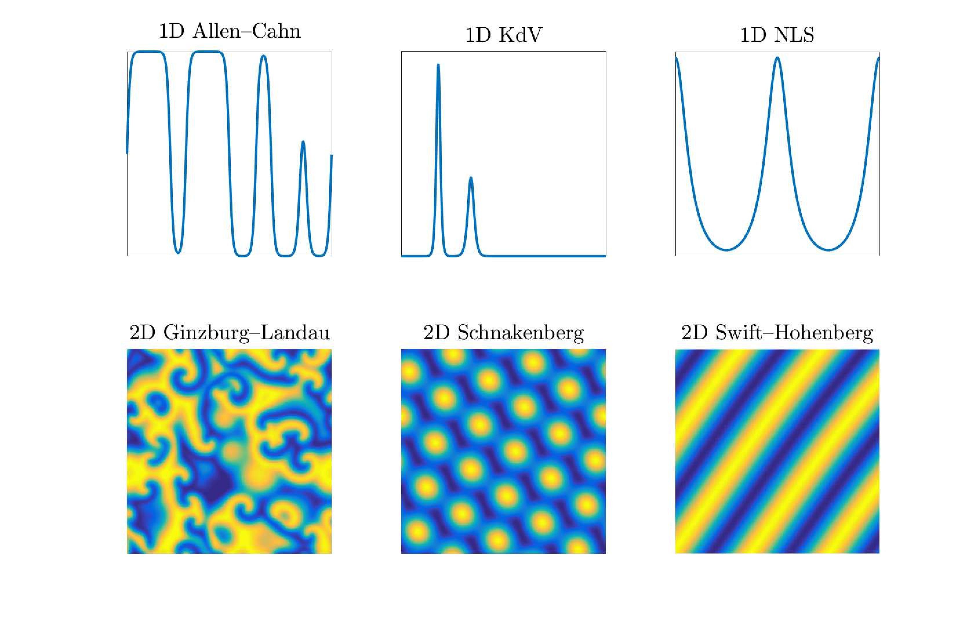
In applications, PDEs of this kind typically arise when two or more different physical processes are combined, and many PDEs of interest in science and engineering take this form. For example, the Korteweg–de Vries equation \(u_t = -u_{xxx} - uu_x\), the starting point of the study of nonlinear waves and solitons, couples third-order linear dispersion with first-order convection, and the Allen–Cahn equation \(u_t = \epsilon u_{xx} + u - u^3\) couples second-order linear diffusion with a nondifferentiated cubic reaction term.
Often a system of equations rather than a single scalar equation is involved, for example in reaction-diffusion systems such as the Gray–Scott and Schnakenberg equations, which involve two components coupled together. (The importance of coupling of nonequal diffusion constants in science was made famous by Alan Turing in 1952 in the most highly-cited of all his papers.) Fourth-order terms also arise, for example in the Cahn–Hilliard equation, whose solutions describe structures of alloys, and in the Kuramoto–Sivashinsky equation, related to combustion problems among others, whose solutions are chaotic. The figure at the top of this post shows six examples of solutions of such PDEs.
Discretization in Fourier space
Our paper describes and compares specialized methods that take advantage of two special features of the family of PDEs above. The first one is the periodic boundary conditions. This allows us to discretize the spatial component with a Fourier spectral method on \(N\) points; the PDE becomes a system of \(N\) ODEs, $$ \widehat{u}' = \mathbf{L}\widehat{u} + \mathbf{N}(\widehat{u}), \quad \widehat{u}(0)=\widehat{u}_0, $$ where \(\widehat{u}(t)\) is the vector of \(N\) Fourier coefficients of the trigonometric interpolant of \(u(t,X)\) at time \(t\), and \(\mathbf{L}\) (a \(N\times N\) matrix) and \(\mathbf{N}\) are the discretized versions of \(\mathcal{L}\) and \(\mathcal{N}\) in Fourier space.
For example, in 1D on \([0, 2\pi]\) with \(\mathcal{L}u=u_{xx}\) and an even number \(N\) of equispaced grid points \(\{x_j=2\pi j/N\}_{j=0}^{N-1}\), we look for a solution \(u(t,x)\) of the form $$ u(t,x) \approx \sum_{k=-N/2}^{N/2}{\hspace{-0.3cm}}'{\;\,} \widehat{u}_k(t) e^{ikx} $$ with Fourier coefficients $$ \widehat{u}_k(t) = \frac{1}{N}\sum_{j=0}^{N-1}u(t,x_j)e^{-ikx_j},\;\; -\frac{N}{2}\leq k\leq \frac{N}{2}-1, $$ and with \(\widehat{u}_{N/2}(t) = \widehat{u}_{-N/2}(t)\). (The prime on the summation sign signifies that the terms \(k=\pm N/2\) are halved.) Since FFT codes only store \(N\) coefficients, the vector \(\widehat{u}(t)\) is defined as $$ \widehat{u}(t) = \Big(\frac{\widehat{u}_{-N/2}}{2}+\frac{\widehat{u}_{N/2}}{2}, \widehat{u}_{-N/2+1}(t),\ldots,\widehat{u}_{N/2-1}(t)\Big)^T. $$ For this PDE, \(\mathbf{L}=\mathbf{D}_N^{(2)}\) is the (diagonal) second-order Fourier differentiation matrix with entries \(-k^2\), \(-N/2\leq k\leq N/2-1\). Note that stiffness is related to \(\mathbf{L}\) having large eigenvalues since the stability of spectral methods for time-dependent PDEs requires that the eigenvalues, scaled by the time-step, lie in the stability region of the time-stepping formula.
A simple exponential integrator
The second special feature of these PDEs is that they are is semilinear, i.e., the higher-order terms of the equation are linear. Exponential integrators are a class of numerical methods for systems of ODEs that are aimed at taking advantage of this. The linear part \(\mathbf{L}\), responsible for the stiffness, is integrated exactly using the matrix exponential while a numerical scheme is applied to \(\mathbf{N}\).
One of the simplest exponential integrators, commonly known as the Exponential Time Differencing (ETD) Euler method, is given by $$ \widehat{u}^{n+1} = e^{h\mathbf{L}}\widehat{u}^n + h\varphi_1(h\mathbf{L})\mathbf{N}(\widehat{u}^n), $$ where \(h=t_{n+1}-t_n\) is the time-step and $$ \varphi_1(z) = \frac{e^z-1}{z}. $$ Note that, in practice, the nonlinear evaluations \(\mathbf{N}(\widehat{u}^n)\) is carried out in value space, that is, \(\mathbf{N}(\widehat{u}^n)\) means \(\mathbf{F}(\mathbf{N}(\mathbf{F}^{-1}\widehat{u}^n))\), with discrete Fourier transform \(\mathbf{F}\). Since the matrix \(\mathbf{L}\) diagonal, computing the matrix exponential and matrix-vector products cost only \(\mathcal{O}(N)\) operations. The dominant cost per time-step is therefore the cost of an FFT, i.e., \(\mathcal{O}(N\log N)\) operations.
Results of our numerical experiments and Chebfun
We compare in our paper 30 exponential integrators of fourth and higher order on 11 model problems in 1D, 2D, and 3D. Our conclusion is that it is hard to do much better than one of the simplest of these formulas, the ETDRK4 scheme of Cox and Matthews.
Our numerical experiments were performed using MATLAB and have been embedded within Chebfun. More specifically, the spin, spin2 and spin3 codes implement a Fourier spectral method and exponential integrators to solve PDEs in 1D, 2D, and 3D periodic domains. The simplest way to see spin in action is to type simply spin('ks') (for the Kuramoto–Sivashinsky equation) or spin2('gl') (for the 2D Ginzburg–Landau equation) to invoke an example computation.
It is also possible to define your own PDE using the spinop class. Check out the documentation for details.
Blog posts about spectral methods
- 2026 A nonlocal Stokes theorem on the sphere
- 2020 Exponential integrators for stiff PDEs
- 2018 Computer-assisted proofs for PDEs
- 2018 Spherical caps in cell polarization
- 2018 Solving nonlocal equations on the sphere
- 2018 Gibbs phenomenon and Cesàro mean
- 2017 Solving PDEs on the sphere
- 2017 When planets dance